US5247461A - Method and apparatus for coincidence correction in electrozone particle sensing - Google Patents
Method and apparatus for coincidence correction in electrozone particle sensing Download PDFInfo
- Publication number
- US5247461A US5247461A US07/738,119 US73811991A US5247461A US 5247461 A US5247461 A US 5247461A US 73811991 A US73811991 A US 73811991A US 5247461 A US5247461 A US 5247461A
- Authority
- US
- United States
- Prior art keywords
- particles
- coincidence
- correction
- sensing
- unit
- Prior art date
- Legal status (The legal status is an assumption and is not a legal conclusion. Google has not performed a legal analysis and makes no representation as to the accuracy of the status listed.)
- Expired - Fee Related
Links
- 239000002245 particle Substances 0.000 title claims abstract description 121
- 238000000034 method Methods 0.000 title claims abstract description 48
- 238000012937 correction Methods 0.000 title claims description 37
- 238000009826 distribution Methods 0.000 claims abstract description 46
- 239000012530 fluid Substances 0.000 claims description 10
- 239000000725 suspension Substances 0.000 claims description 9
- 239000007788 liquid Substances 0.000 claims description 3
- 238000010790 dilution Methods 0.000 claims 1
- 239000012895 dilution Substances 0.000 claims 1
- 230000000694 effects Effects 0.000 description 17
- 230000008569 process Effects 0.000 description 16
- 238000004364 calculation method Methods 0.000 description 9
- 230000004044 response Effects 0.000 description 8
- 238000004062 sedimentation Methods 0.000 description 8
- 238000004458 analytical method Methods 0.000 description 7
- 238000003921 particle size analysis Methods 0.000 description 7
- 102100023705 C-C motif chemokine 14 Human genes 0.000 description 5
- 101100382874 Homo sapiens CCL14 gene Proteins 0.000 description 5
- 230000008901 benefit Effects 0.000 description 5
- 238000001514 detection method Methods 0.000 description 4
- 238000005259 measurement Methods 0.000 description 4
- 230000003287 optical effect Effects 0.000 description 4
- 238000003491 array Methods 0.000 description 3
- 230000005684 electric field Effects 0.000 description 3
- 239000003792 electrolyte Substances 0.000 description 3
- 239000000463 material Substances 0.000 description 3
- 238000001228 spectrum Methods 0.000 description 3
- 101100132477 Arabidopsis thaliana NAC69 gene Proteins 0.000 description 2
- 102100023703 C-C motif chemokine 15 Human genes 0.000 description 2
- 101100382875 Homo sapiens CCL15 gene Proteins 0.000 description 2
- 238000006073 displacement reaction Methods 0.000 description 2
- 230000010354 integration Effects 0.000 description 2
- 230000009467 reduction Effects 0.000 description 2
- 238000000926 separation method Methods 0.000 description 2
- 238000010521 absorption reaction Methods 0.000 description 1
- 238000007792 addition Methods 0.000 description 1
- 239000000654 additive Substances 0.000 description 1
- 230000000996 additive effect Effects 0.000 description 1
- 238000013459 approach Methods 0.000 description 1
- 238000000149 argon plasma sintering Methods 0.000 description 1
- 230000008859 change Effects 0.000 description 1
- 239000002131 composite material Substances 0.000 description 1
- 238000005520 cutting process Methods 0.000 description 1
- 230000008030 elimination Effects 0.000 description 1
- 238000003379 elimination reaction Methods 0.000 description 1
- 238000013213 extrapolation Methods 0.000 description 1
- 239000012634 fragment Substances 0.000 description 1
- 230000006870 function Effects 0.000 description 1
- 230000014509 gene expression Effects 0.000 description 1
- 238000007654 immersion Methods 0.000 description 1
- 238000011835 investigation Methods 0.000 description 1
- 230000001788 irregular Effects 0.000 description 1
- 239000011159 matrix material Substances 0.000 description 1
- 238000002156 mixing Methods 0.000 description 1
- 238000012986 modification Methods 0.000 description 1
- 230000004048 modification Effects 0.000 description 1
- 238000012544 monitoring process Methods 0.000 description 1
- 230000000704 physical effect Effects 0.000 description 1
- 238000002360 preparation method Methods 0.000 description 1
- 230000009290 primary effect Effects 0.000 description 1
- 238000012545 processing Methods 0.000 description 1
- 238000010223 real-time analysis Methods 0.000 description 1
- 238000011084 recovery Methods 0.000 description 1
- 238000005070 sampling Methods 0.000 description 1
- 230000009291 secondary effect Effects 0.000 description 1
- 230000035945 sensitivity Effects 0.000 description 1
- 238000004513 sizing Methods 0.000 description 1
- 239000012798 spherical particle Substances 0.000 description 1
- 230000007480 spreading Effects 0.000 description 1
- 238000003892 spreading Methods 0.000 description 1
- 238000003860 storage Methods 0.000 description 1
Images
Classifications
-
- G01N15/132—
-
- G—PHYSICS
- G01—MEASURING; TESTING
- G01N—INVESTIGATING OR ANALYSING MATERIALS BY DETERMINING THEIR CHEMICAL OR PHYSICAL PROPERTIES
- G01N15/00—Investigating characteristics of particles; Investigating permeability, pore-volume, or surface-area of porous materials
- G01N15/10—Investigating individual particles
- G01N15/1031—Investigating individual particles by measuring electrical or magnetic effects thereof, e.g. conductivity or capacity
-
- G—PHYSICS
- G01—MEASURING; TESTING
- G01N—INVESTIGATING OR ANALYSING MATERIALS BY DETERMINING THEIR CHEMICAL OR PHYSICAL PROPERTIES
- G01N15/00—Investigating characteristics of particles; Investigating permeability, pore-volume, or surface-area of porous materials
- G01N15/10—Investigating individual particles
- G01N15/1012—Calibrating particle analysers; References therefor
-
- G01N2015/1024—
-
- G01N2015/1029—
Definitions
- This invention relates to a method of obtaining an accurate representation of the size distribution of particles in a fluid sample, using a conventional particle detecting apparatus.
- Electrozone sensing responds to the displacement volume of each particle as the amplitude of its electrical pulse, thus providing the basis for electrozone particle size analysis (PSA) via a frequency histogram.
- PSA electrozone particle size analysis
- the electrozone method In automated particle size analysis, the electrozone method has three intrinsic advantages in the elements of precision; true size sensing, low side effects and simplicity. These result in response purity and sensing reliability that make it naturally superior to the other major automated methods, sedimentation and various light beam interference methods including forward scatter, obscuration, diffraction and beam transit time.
- the precision that is possible with the electrozone method provides the highest quality of measurement fidelity and hence a unique possibility for mathematical elimination of coincidence effects that produce unacceptable data distortion.
- the electrozone principle has three intrinsic advantages over the sedimentation or light beam interference methods which make it uniquely able to utilize rigorous mathematics for distributional coincidence correction.
- the truest measure of particle size sensing the displacement volumes of individual particles in an electrical field, with the proportionality being true to a fraction of a percent from less than 0.5 to more than 1000 micrometers.
- Light beam interference methods are greatly affected by shape as well as refractive index, opacity and absorption. Sedimentation is also highly sensitive to particle shape, as well as particle density, optical properties (when using light beams), and to liquid (or gas) density, convection and viscosity (note falling ball or falling needle viscometers).
- Electrozone employs merely a simple hole vs. a multi-instrument sensor for the said other major methods: beam source, optical train, photic receptor, plus (in sedimentation) a temperature/convection control system, plus (when accelerated) a centrifuge control system.
- Electrozone calibration may be general (accurate to within a few percent) or of pin-point precision through easily used standard particles, narrowly distributed. Precise calibration allows accuracy within a few tenths of one percent (stating size as "volume equivalent spherical diameter").
- Calibrations for sedimentation and light beam interference methods are done by theoretical response equations or by the use of specific materials having known distributions or by narrowly distributed standards. Data blurring, due to the compromises of side effects and multi-particle response as described above, is evidenced, e.g., by a marked spreading of the distributions for narrowly sized standards. Because of the compromises, these area sensing methods can only be calibrated for specific applications.
- PDC particle dedicated to coincidence
- the total coincidence effect on the entire population is a net loss of particle count.
- the distributed coincidence effect is the gain and/or loss of count at every increment or channel of particle size.
- the algebraic sum of the distributed coincidence throughout the population equals the total coincidence.
- Particle concentration, electrolyte conductivity, orifice size, and electric field gradient are selected to cause a sequence of measurable particle pulses each pulse defined by a rise from and return to an electrical level set above a steady state base line.
- Each pulse represents a passage of a single particle or the coincidence passage of two or more particles. Pulse amplitude for a single particle is proportional to its volume, enabling precise size analysis for suspensions that are dilute enough to ensure virtually no coincidence.
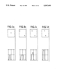
- FIGS. 1A-1D For multi-particle passages, the pulses are superimposed signals having amplitudes ranging from that for the largest particle to the sum of the amplitudes for the coincidence particles, it is illustrated in FIGS. 1A-1D.
- FIG. 1A illustrates a cross sectional view of an orifice at the time a single particle passes through it, with the resulting pulse which is produced.
- FIG. 1B illustrates a condition in which two particles, widely separated, are present in the orifice at the same time, with the modified pulse it results therefrom.
- FIG. 1D illustrates a condition in which the two particles pass through the orifice in nearly side-by-side condition, with the resulting pulse, and
- FIG. 1C shows the condition intermediate the conditions of FIGS. 1B and 1D.
- the primary effect is a loss of count for the particle population, due to the undetected particles in multi-particle pulses.
- the secondary effect due to the spurious pulse amplitudes for coincidence passages and the missing single particle pulses, is distortion of the size distribution data, shifting it toward the larger diameter particles.
- the present invention uses means for accelerated generation of a pseudo-function that is negligibly different from that generated by a lengthy integration process, but is much more rapidly obtained.
- the observed PSA histogram which is sometimes hereinafter referred to as a first approximation, has embedded within it both a true particle size distribution and a spurious distribution of coincidence-formed pulses. This invention allows clear separation of the spurious distribution and from this the generation of a complete, true distribution.
- the proximity of two particles, A and B then ranges from the minimum proximity where A precedes B, to the maximum proximity of exact superimposition, to the minimum proximity where B precedes A.
- the additive signal caused by superposition of the pulses has five phases:
- the PDC originates the pseudo-distribution which thus must be found by computing it from the PDC.
- the true distribution is unknown, so the observed distribution is used as the approximate shape of the PDC distribution.
- the total PDC count quantity is calculated from Poisson statistics.
- the pseudo-distribution is determined by computing and summing, for each channel of the PDC distribution, the probabilities of all of the possible combinations of particles forming that channel.
- the computation of count loss due to coincidence is based on the Poisson distribution of the particles in the suspension.
- the computation of the distribution distortion is much more complex. It is a principal object of the present invention to correct for distortion in the particle size distribution.
- the present invention contemplates the actual distribution of the various sizes of particles in a major population, and the effects of possible particle combinations in binary and tertiary coincidences.
- a binary coincidence is one in which two particles pass through the orifice at the same time
- a tertiary coincidence is one in which three particles are present in the orifice at the same time.
- the probability of having four or more particles present in the orifice at the same time is quite low under practical measuring conditions, so that the conditions of coincidence of four or more particles may be neglected without loss of precision.
- the present invention also considers the probability of all possible degrees of additivity of the component particle signals in the coincidences.
- the present invention also considers the probability of missing pulses, both single and multiple particle pulses, which may otherwise occur during the dead time following each pulse, devoted to recovery of signal processing electronics.
- the present invention accomplishes several benefits.
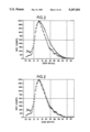
- the 95-98 percent time reduction for data acquisition means an equal reduction of background noise in the data set (see FIGS. 2 and 3).
- Background noise is proportional to sampling time and therefore electrolyte volume (fine debris).
- FIG. 2 illustrates two histogram plots, comparing data from a sample with relatively few coincidences, with data from a sample of the same material with a large number of coincidences, which data have been corrected in accordance with the present invention
- FIG. 3 illustrate two histogram plots indicating raw (first approximation) data and the same data which have been corrected in accordance with the present invention
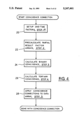
- FIG. 4 is a flow chart illustrating the method of the present invention.
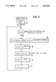
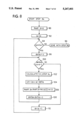
- FIG. 5 is a flowchart of steps performed during step 2 of the process of FIG. 4;
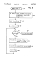
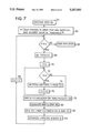
- FIGS. 6 and 7 are first and second portions of the third step of the process of FIG. 4;
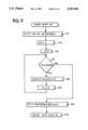
- FIG. 8 is a flowchart of one of the steps of the process of FIG. 7;
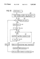
- FIG. 9 is a flowchart of one of the steps of the process of FIG. 8;
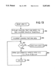
- FIG. 10 is a flowchart of step 4 of the process of FIG. 4;
- FIG. 11 is a flowchart of one of the steps of the process of FIG. 10;
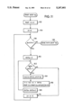
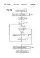
- FIG. 12 is a flowchart of one of the steps of the process of FIG. 11.
- FIG. 13 is a flowchart of the process of step 5 of FIG. 4.
- raw and corrected data taken from a sample having a relatively large number of coincidences, on the order of 20%, are illustrated in two curves, each of which is a histogram plotting particle diameter along the x-axis relative to the number of counts of particles of each size category along the y-axis.
- the curve 10 is the uncorrected curve
- the curve 12 is the curve which has been corrected in accordance with the present invention, which represents the true particle distribution.
- the curve 10 is skewed rightwardly, toward large particles, because the coincidence of multiple particles within the sensing zone gives an indication of a larger particle than any one of the individual particles which are coincident.
- the total number of counts, which is the integral of the curve is smaller for the uncorrected data, since those particles which are included in the coincidences are not counted, which occur during the coincidence period.
- FIG. 2 illustrates the precision of the correction effected by the present invention.
- Curve 14 is the data taken from a relatively dilute sample, in which very few coincidences occur, on the order of 0.5%.
- the curve 16 is corrected data taken from the sample of the same particle distribution, in which a relatively large number of coincidences occur, on the order of 20%.
- the present invention effects a very exact correction of the data, which corresponds closely to data taken from a sample with very few coincidences. Further, the noise at the small end of the high concentration sample is much less, as aforesaid.
- Equation 1 An overview of the correction is expressed by Equation 1: ##EQU1## Where:
- n is the channel number being corrected
- C is the total number of channels, e.g. 128
- NCC[n] is the corrected size histogram array
- NTM[n] is the measured size histogram array
- NP2[n] is the binary pseudo-spectrum array
- NP3[n] is the tertiary pseudo-spectrum array
- FC is the fraction of particles in coincidence in the measured volume, expanded to include deadtime.
- the form of the binary array results from the detailed summing of all coincident size pairings (as extracted from elements of the PDC array, together with their associated probabilities) and the probabilistic effect of composite signal detection as they contribute count to a particular channel [n].
- the tertiary array is produced by a recursion-like process, applied to the already computed binary array, which produces tertiary coincidence.
- NP2 the number of counts to be added or subtracted for channel [n]
- NT2 the estimated number of singlets in the doublet PDC array.
- f a signal detection parameter, 0 ⁇ f ⁇ 1
- Equation 3 The tertiary array is expressed by Equation 3. ##EQU5## Wherein: Many terms are as defined above, but note that for this array, P1, P2[n], P3[n], CC and f definitions are modified.
- NP3 the number of counts to be added or subtracted for channel [n]
- NT total number of particles in expanded volume
- Vs measured volume, without deadtime volume
- VT total (expanded) volume, including deadtime
- NT3 the estimated number of singlet particles in the tertiary PDC array ##EQU6## Terms g( ⁇ ) through ff are as defined for Equation 2.
- FIG. 4 illustrates the steps performed in the process of the present invention. It is convenient to perform the process by programming a general purpose digital computer to perform the steps in sequence. When a readily available computer is used for this purpose, the entire process takes less than one minute, so that the present invention can effectively be used in real time monitoring situations.
- step 1 constants and temporary variables used throughout the remainder of the process are calculated and stored. These factors are either optional constants or fixed constants.
- Optional constants include the number of channels into which the data is distributed, viz., the number of adjacent particle size bands in the histogram. Fixed constants include sensing volume, and the like, which are closely linked to the characteristics of the equipment which is not readily modifiable. The optional constants may be selected by an operator. Thus, the number of channels may be varied in order to provide a coarse or fine resolution in a histogram.
- arrays are typically defined and memory is allocated so that intermediate calculated values can be stored in array or matrix form. This occurs in unit 20, which performs step 1.
- NT (mc * VT/Vs) * (1+td/tm)
- FC2 e -m * m 2 /(2 * (1-e -m ))
- NCC2[i] NT2/(NTM * NTM[i])
- NCC3[i] NT3/(NTM * NTM[i])
- Part 1 is the same for each value, i.e, each particle size.
- Parts 2 and 3 are individual to each size: ##EQU9##
- the binary and tertiary correction are each calculated, for each value, as:
- the arrays typically contain one element or storage location for each of the channels participating in the calculation of the partial results, so that intermediate results can be stored easily.
- the corrected data may be displayed in the form of a histogram, either with a video monitor connected to the computer, or with a printout in the form of a histogram produced by a printer or plotter or the like.
- Unit 30 first receives control, which sets initial values to zero.
- the parameter i is an index, and the initial (zero) component of array A is set to zero.
- unit control passes to unit 32, which determines whether the index i is less than the value Ca. If not, control passes via path 34 to unit 46 of FIG. 6, described hereinafter. Otherwise, control passes to unit 36, which calculates and stores a result in element i of array g. Then control passes to unit 38, where another calculation is performed with the result stored in element i of array b. Then the contents of array g are read out and stored in array A, with the index of array A being one less than the source of the data in array g.
- the value Ca is a value which is calculated in step 1, and represents the range over which the first approximation data are adjusted, for each channel.
- control passes to unit 46, which calculates the parameter dwTotal. Then control passes to unit 48, which calculates "part 1", of the binary correction. Then control passes to unit 50, which sets the index i 0, then control passes to unit 52, which determines whether i has been increased to equal the total number of channels. If so, control passes over path 54 to FIG. 7. Otherwise, unit 56 receives control, and performs a calculation and stores the result in element i of array NCC2. Then unit 58 receives control, and performs a calculation, and stores the result in element i of array NCC3. Then unit 60 increments i and returns the control to unit 52. Thus, before control passes to FIG. 7, the loop of units 52-60 has been repeated for each of the total number of channels.
- unit 78 calculates "part 2" of the binary correction, and then unit 80 calculates "part 3" of the binary correction; and then control passes to unit 82 which stores a calculated value derived from parts 1, 2 and 3 in element n of array NP2. Then control passes to unit 84, which makes a calculation and stores the result in element n of array NP23. The contents of the array NP23 are used for tertiary compensation, described hereinafter. Then control passes to unit 88, which decrements the value of n, and returns control to unit 64.
- FIG. 8 illustrates the units incorporated in the unit 80 of FIG. 7.
- the unit 90 receives control from unit 78 (FIG. 7), and sets the initial value of "part 3" of the binary correction equal to zero. Then unit 92 sets an index parameter a equal to zero, and passes control to unit 94. The unit 94 determines whether a is greater than the value of Ca-1, and if so, passes control to an exit which in turn passes control back to unit 82 (FIG. 7). Otherwise, unit 98 receives control which sets a parameter "delta" equal to an initial value of zero. Then unit 100 determines whether the current value of delta is greater than Ca-a-1, and if so, passes control unit 110, which increments A and returns control to unit 94. Otherwise, control passes to unit 102, which calculates the value CC.
- unit 104 calculates an index i, which is used to access element i of the array NCC2, by unit 106, which receives control next. Then control passes to unit 108, which increments the value of delta and returns control to the unit 100. The loop incorporating units 100-108 is repeated until delta is increased to a value which exceeds Ca-a-1.
- unit 102 The components of unit 102 are illustrated in FIG. 9.
- FIG. 9 receives control from unit 100, for low values of delta, and control passes to unit 112, which computes a value for w (used by unit 120), after which indexes dl and i are set to zero by units 114 and 116. Then unit 118 determines whether i has been increased to a value which exceeds the delta component of array A, and if so, control passes to unit 124. Otherwise, control passes to unit 120, which calculates the value for dl by increasing the previous value of dl by the content of one of the elements of the array NCC2, namely, element w+1. Then the index i is incremented in unit 122, and control returns to unit 118. The loop incorporating units 118-122 is repeated until i exceeds the delta component of array A.
- Unit 124 calculates the value for CC, and returns control to unit 104 (FIG. 8) over path 126.
- unit 26 of FIG. 4 which calculates the tertiary correction factor, are illustrated in FIG. 10.
- Unit 128 receives the control first, which recalculates the value of n, which is the same value of n calculated in unit 62 of FIG. 7. Then unit 130 receives control, which determines whether the value of n is less than zero, and if so, control passes over path 132 to unit 28 of FIG. 4. Otherwise, unit 134 sets the initial value of dwTotal equal to zero, and index i equal to zero, in units 134 and 136. Then units 138-142 perform a loop corresponding to the loop of units 72-76 of FIG. 7, after which units 144 and 146 calculate "part 2" and "part 3" for the tertiary correction, and unit 148 calculates the final tertiary correction and stores it in element n of array NP3. Then unit 150 decrements n and returns control to unit 130.
- unit 146 The components of unit 146 are illustrated in FIG. 11.
- the components of FIG. 11 incorporate units 152-170, which correspond with units 90-110 of FIG. 8.
- the units of FIG. 11 calculate "part 3" of the tertiary coincidence, while the corresponding units of FIG. 8 calculate "part 3" of the binary coincidence.
- unit 164 The components of unit 164 are illustrated in FIG. 12.
- Units 172-184 of FIG. 4 correspond to units 112-124 of FIG. 9, except that the units of FIG. 12 calculates CC for the tertiary coincidence, while the corresponding units of FIG. 9 make the calculation for the binary coincidence.
- FIG. 13 illustrates the components of unit 28.
- Control passes first to unit 186, which again calculates the value n which is the same as the value calculated in units 62 and 128. Then the index i is set by unit 188 to the lowest channel that has data, and control passes to unit 190. If i is not less than n, control passes to an exit over path 192, and the correction process is complete. Otherwise, control passes to unit 194, which adjusts the element i of the array A in accordance with the binary coincidence correction stored in element i of array NP2, and the tertiary coincidence correction stored in element i of array NP3. Then unit 196 increments i and returns control to unit 190. The loop including units 190-196 is repeated until all of the elements of the array which contain data have been adjusted to account for the binary and tertiary coincidence correction.
- the present invention affords a simple and effective means of modifying particle count data to correct for coincidences.
- the entire operation is performed rapidly, and results in data which represents an precise particle distribution histogram of the sample under investigation, irrespective of its concentration, i.e., independent of the number of coincidences actually experienced within the sensing zone.
- the use of the present invention makes it unnecessary to modify samples to reduce the proportion of coincidences, since the presence of coincidence does not result in inaccurate data.
- the present invention also makes it possible to perform the coincidence corrections sufficiently rapidly so that dynamic conditions may be investigated in real time.
Abstract
Description
              TABLE 1
______________________________________
Initial Constants
______________________________________
C          number of channels of data in the
           distribution.
Vs         Sensing volume, the amount of fluid that is
           present in the sensor zone.
VT         total volume of fluid run through the sensor.
tm         measuring time.
td         dead time of the sensor electronics
f and ff   signal detection parameters
Array [N]  measured size histogram as produced by
           instrument, at end of procedure, updated to
           show the true corrected count
______________________________________
NP2[n]=Part 1 * (KI * Part 2[n]+K2 * Part 3[n])
Claims (6)
Priority Applications (1)
| Application Number | Priority Date | Filing Date | Title |
|---|---|---|---|
| US07/738,119 US5247461A (en) | 1991-07-30 | 1991-07-30 | Method and apparatus for coincidence correction in electrozone particle sensing |
Applications Claiming Priority (1)
| Application Number | Priority Date | Filing Date | Title |
|---|---|---|---|
| US07/738,119 US5247461A (en) | 1991-07-30 | 1991-07-30 | Method and apparatus for coincidence correction in electrozone particle sensing |
Publications (1)
| Publication Number | Publication Date |
|---|---|
| US5247461A true US5247461A (en) | 1993-09-21 |
Family
ID=24966655
Family Applications (1)
| Application Number | Title | Priority Date | Filing Date |
|---|---|---|---|
| US07/738,119 Expired - Fee Related US5247461A (en) | 1991-07-30 | 1991-07-30 | Method and apparatus for coincidence correction in electrozone particle sensing |
Country Status (1)
| Country | Link |
|---|---|
| US (1) | US5247461A (en) |
Cited By (10)
| Publication number | Priority date | Publication date | Assignee | Title |
|---|---|---|---|---|
| US5452237A (en) * | 1994-02-28 | 1995-09-19 | Abbott Laboratories | Coincidence error correction system for particle counters |
| US6122599A (en) * | 1998-02-13 | 2000-09-19 | Mehta; Shailesh | Apparatus and method for analyzing particles |
| US20030020447A1 (en) * | 2001-07-27 | 2003-01-30 | Taylor Richard Lee | Particle count correction method and apparatus |
| US20030073136A1 (en) * | 2001-10-17 | 2003-04-17 | Gerd Luedke | Method of and apparatus for performing flow cytometric measurements |
| US20050249411A1 (en) * | 2004-05-04 | 2005-11-10 | Metso Automation Oy | Generation of frequency distribution for objects |
| US20140268102A1 (en) * | 2013-03-14 | 2014-09-18 | Abbott Laboratories | Methods for Detecting Coincident Sample Events, and Devices and Systems Related Thereto |
| CN106769698A (en) * | 2016-12-29 | 2017-05-31 | 长春迪瑞医疗科技股份有限公司 | A kind of haemocyte abnormal pulsers signal identification processing method based on theory of electrical impedance |
| US20170328825A1 (en) * | 2015-07-14 | 2017-11-16 | Teilch Llc | Airborne particle measuring device |
| WO2022195994A1 (en) * | 2021-03-18 | 2022-09-22 | 株式会社Jvcケンウッド | Analysis device and analysis method |
| US11789166B2 (en) * | 2019-06-25 | 2023-10-17 | Aerosol Dynamics Inc. | Pulse counting coincidence correction based on count rate and measured live time |
Citations (6)
| Publication number | Priority date | Publication date | Assignee | Title |
|---|---|---|---|---|
| US3626164A (en) * | 1968-06-19 | 1971-12-07 | Coulter Electronics | Digitalized coincidence correction method and circuitry for particle analysis apparatus |
| GB2033119A (en) * | 1978-09-29 | 1980-05-14 | Hycel Inc | Particle analysis |
| US4447883A (en) * | 1981-05-26 | 1984-05-08 | Technicon Instruments Corporation | Coincidence-error correcting apparatus and method |
| US4488248A (en) * | 1980-12-05 | 1984-12-11 | Toa Medical Electronics Co., Ltd. | Particle size distribution analyzer |
| US4510438A (en) * | 1982-02-16 | 1985-04-09 | Coulter Electronics, Inc. | Coincidence correction in particle analysis system |
| US4612614A (en) * | 1980-09-12 | 1986-09-16 | International Remote Imaging Systems, Inc. | Method of analyzing particles in a fluid sample |
-
1991
- 1991-07-30 US US07/738,119 patent/US5247461A/en not_active Expired - Fee Related
Patent Citations (6)
| Publication number | Priority date | Publication date | Assignee | Title |
|---|---|---|---|---|
| US3626164A (en) * | 1968-06-19 | 1971-12-07 | Coulter Electronics | Digitalized coincidence correction method and circuitry for particle analysis apparatus |
| GB2033119A (en) * | 1978-09-29 | 1980-05-14 | Hycel Inc | Particle analysis |
| US4612614A (en) * | 1980-09-12 | 1986-09-16 | International Remote Imaging Systems, Inc. | Method of analyzing particles in a fluid sample |
| US4488248A (en) * | 1980-12-05 | 1984-12-11 | Toa Medical Electronics Co., Ltd. | Particle size distribution analyzer |
| US4447883A (en) * | 1981-05-26 | 1984-05-08 | Technicon Instruments Corporation | Coincidence-error correcting apparatus and method |
| US4510438A (en) * | 1982-02-16 | 1985-04-09 | Coulter Electronics, Inc. | Coincidence correction in particle analysis system |
Cited By (20)
| Publication number | Priority date | Publication date | Assignee | Title |
|---|---|---|---|---|
| US5452237A (en) * | 1994-02-28 | 1995-09-19 | Abbott Laboratories | Coincidence error correction system for particle counters |
| US6122599A (en) * | 1998-02-13 | 2000-09-19 | Mehta; Shailesh | Apparatus and method for analyzing particles |
| US6426615B1 (en) | 1998-02-13 | 2002-07-30 | Shailesh Mehta | Apparatus and method for analyzing particles |
| US20030020447A1 (en) * | 2001-07-27 | 2003-01-30 | Taylor Richard Lee | Particle count correction method and apparatus |
| WO2003012418A1 (en) | 2001-07-27 | 2003-02-13 | Coulter International Corp. | Particle count correction method and apparatus |
| US6744245B2 (en) * | 2001-07-27 | 2004-06-01 | Coulter International Corp. | Particle count correction method and apparatus |
| US20030073136A1 (en) * | 2001-10-17 | 2003-04-17 | Gerd Luedke | Method of and apparatus for performing flow cytometric measurements |
| EP1304557A1 (en) * | 2001-10-17 | 2003-04-23 | Agilent Technologies, Inc. (a Delaware corporation) | Method of performing flow cytometric measurements and apparatus for performing the method |
| US20050249411A1 (en) * | 2004-05-04 | 2005-11-10 | Metso Automation Oy | Generation of frequency distribution for objects |
| US8515151B2 (en) * | 2004-05-04 | 2013-08-20 | Metso Automation Oy | Generation of frequency distribution for objects |
| US20140268102A1 (en) * | 2013-03-14 | 2014-09-18 | Abbott Laboratories | Methods for Detecting Coincident Sample Events, and Devices and Systems Related Thereto |
| US9335246B2 (en) * | 2013-03-14 | 2016-05-10 | Abott Laboratories | Methods for detecting coincident sample events, and devices and systems related thereto |
| US9638623B2 (en) | 2013-03-14 | 2017-05-02 | Abbott Laboratories | Methods for detecting coincident sample events, and devices and systems related thereto |
| US11150176B2 (en) | 2013-03-14 | 2021-10-19 | Abbott Laboratories | Methods for detecting coincident sample events, and devices and systems related thereto |
| US20170328825A1 (en) * | 2015-07-14 | 2017-11-16 | Teilch Llc | Airborne particle measuring device |
| US10151682B2 (en) * | 2015-07-14 | 2018-12-11 | Teilch Llc | Airborne particle measuring device |
| CN106769698A (en) * | 2016-12-29 | 2017-05-31 | 长春迪瑞医疗科技股份有限公司 | A kind of haemocyte abnormal pulsers signal identification processing method based on theory of electrical impedance |
| CN106769698B (en) * | 2016-12-29 | 2019-08-06 | 迪瑞医疗科技股份有限公司 | A kind of haemocyte abnormal pulsers signal identification processing method based on theory of electrical impedance |
| US11789166B2 (en) * | 2019-06-25 | 2023-10-17 | Aerosol Dynamics Inc. | Pulse counting coincidence correction based on count rate and measured live time |
| WO2022195994A1 (en) * | 2021-03-18 | 2022-09-22 | 株式会社Jvcケンウッド | Analysis device and analysis method |
Similar Documents
| Publication | Publication Date | Title |
|---|---|---|
| Harris et al. | Automated quantification of roots using a simple image analyzer | |
| US5247461A (en) | Method and apparatus for coincidence correction in electrozone particle sensing | |
| EP0201849B1 (en) | Method and apparatus for dimensional analysis of continuously produced tubular objects | |
| Brenguier et al. | Improvements of droplet size distribution measurements with the Fast-FSSP (Forward Scattering Spectrometer Probe) | |
| US6542234B1 (en) | Method of detecting the particles of a tobacco particle stream | |
| JP3081270B2 (en) | Analytical instrument and its calibration method | |
| KR101283220B1 (en) | Radiation detector and radiation detecting method | |
| JPH0410034B2 (en) | ||
| US4596464A (en) | Screening method for red cell abnormality | |
| EP1711800B1 (en) | Method and device for determining the material of an object | |
| MXPA97006597A (en) | Method for the regulation and discrimination of the form of the impulse in a nucl spectroscopy system | |
| EP0998137A2 (en) | Method and apparatus for defective pixel identification | |
| Pover et al. | Verification of the disector method for counting neurons, with comments on the empirical method | |
| EP1349879B1 (en) | System and method for determining molecular weight and intrinsic viscosity of a polymeric distribution using gel permeation chromatography | |
| US4510438A (en) | Coincidence correction in particle analysis system | |
| Ashenden et al. | Standardization of reticulocyte values in an antidoping context | |
| Benveniste et al. | The problem of measuring the absolute yield of 14-MeV neutrons by means of an alpha counter | |
| US3949198A (en) | Methods and apparatuses for correcting coincidence count inaccuracies in a coulter type of particle analyzer | |
| CN110088605A (en) | The method of adjustment of X-ray analysis signal processing apparatus and X-ray analysis signal processing apparatus | |
| US4309757A (en) | Method for classification of signals by comparison with an automatically determined threshold | |
| Röver et al. | Indirect determination of leaf area index of sugar beet canopies in comparison to direct measurement | |
| Peacock et al. | Instrumental effects in quantitative Auger electron spectroscopy | |
| Hine | Evaluation of focused collimator performance II. Digital recording of line-source response | |
| EP0138591A2 (en) | Screening method for red blood cell abnormality | |
| US5166964A (en) | Method and apparatus for measuring density |
Legal Events
| Date | Code | Title | Description |
|---|---|---|---|
| AS | Assignment |
Owner name: PARTICLE DATA, INC., A CORP. OF IL Free format text: ASSIGNMENT OF ASSIGNORS INTEREST.;ASSIGNOR:BAKALYAR, GEORGE A.;REEL/FRAME:005861/0681 Effective date: 19910925 Owner name: PARTICLE DATA, INC., ILLINOIS Free format text: ASSIGNMENT OF ASSIGNORS INTEREST.;ASSIGNOR:BERG, ROBERT H.;REEL/FRAME:005861/0665 Effective date: 19910929 |
|
| FEPP | Fee payment procedure |
Free format text: PAT HOLDER CLAIMS SMALL ENTITY STATUS - SMALL BUSINESS (ORIGINAL EVENT CODE: SM02); ENTITY STATUS OF PATENT OWNER: SMALL ENTITY |
|
| REMI | Maintenance fee reminder mailed | ||
| FPAY | Fee payment |
Year of fee payment: 4 |
|
| SULP | Surcharge for late payment | ||
| LAPS | Lapse for failure to pay maintenance fees | ||
| AS | Assignment |
Owner name: MICROMERITICS INSTRUMENT CORPORATION, GEORGIA Free format text: ASSIGNMENT OF ASSIGNORS INTEREST;ASSIGNOR:PARTICLE DATA, INC.;REEL/FRAME:008761/0949 Effective date: 19970725 |
|
| FP | Lapsed due to failure to pay maintenance fee |
Effective date: 19970924 |
|
| FEPP | Fee payment procedure |
Free format text: PAYOR NUMBER ASSIGNED (ORIGINAL EVENT CODE: ASPN); ENTITY STATUS OF PATENT OWNER: SMALL ENTITY |
|
| FEPP | Fee payment procedure |
Free format text: PAYER NUMBER DE-ASSIGNED (ORIGINAL EVENT CODE: RMPN); ENTITY STATUS OF PATENT OWNER: SMALL ENTITY Free format text: PAYOR NUMBER ASSIGNED (ORIGINAL EVENT CODE: ASPN); ENTITY STATUS OF PATENT OWNER: SMALL ENTITY |
|
| STCH | Information on status: patent discontinuation |
Free format text: PATENT EXPIRED DUE TO NONPAYMENT OF MAINTENANCE FEES UNDER 37 CFR 1.362 |