US5408598A - Method for fast generation of parametric curves employing a pre-calculated number of line segments in accordance with a determined error threshold - Google Patents
Method for fast generation of parametric curves employing a pre-calculated number of line segments in accordance with a determined error threshold Download PDFInfo
- Publication number
- US5408598A US5408598A US08/202,678 US20267894A US5408598A US 5408598 A US5408598 A US 5408598A US 20267894 A US20267894 A US 20267894A US 5408598 A US5408598 A US 5408598A
- Authority
- US
- United States
- Prior art keywords
- sub
- curve
- error value
- error
- computing
- Prior art date
- Legal status (The legal status is an assumption and is not a legal conclusion. Google has not performed a legal analysis and makes no representation as to the accuracy of the status listed.)
- Expired - Fee Related
Links
Images
Classifications
-
- G—PHYSICS
- G06—COMPUTING; CALCULATING OR COUNTING
- G06T—IMAGE DATA PROCESSING OR GENERATION, IN GENERAL
- G06T11/00—2D [Two Dimensional] image generation
- G06T11/20—Drawing from basic elements, e.g. lines or circles
- G06T11/203—Drawing of straight lines or curves
-
- G—PHYSICS
- G06—COMPUTING; CALCULATING OR COUNTING
- G06F—ELECTRIC DIGITAL DATA PROCESSING
- G06F17/00—Digital computing or data processing equipment or methods, specially adapted for specific functions
- G06F17/10—Complex mathematical operations
- G06F17/17—Function evaluation by approximation methods, e.g. inter- or extrapolation, smoothing, least mean square method
Definitions
- This invention relates to computer graphics, and more precisely, to a method and apparatus for rapidly generating curves on a computer display.
- Computer graphics employ a number of techniques to reproduce curved lines and surfaces.
- One commonly used technique involves producing a set of points and connecting those points with straight lines to approximate the curve. The curve is successively divided into smaller pieces and then checked to see if each piece can be approximated by a straight line to within a given error threshold. It turns out that the check of the accuracy of the approximation is the dominant part of the cost of executing the curve approximation algorithm.
- a curve In a two-dimensional space, a curve is often expressed as a function of orthogonal components x and y, i.e., y is equal to f(x).
- the x, y and z coordinates may also be represented as functions of one or two of the orthogonal components. However, these representations may cause difficulty in generating the coordinate values.
- One alternative technique is to use a parametric representation of the curve or a representation where each coordinate value on a curve is represented as a function of some common variable, that is, a variable common to all coordinate components.
- a further representation is a parametric cubic curve that is represented by third order polynomials.
- Cubic curves are important because no lower-order representation of curve segments can provide either continuity of position and slope or continuity of slope and curvature at the point where the curve segments meet. Cubic curves are also the lowest order curves that can render non-planar curves in three dimensions.
- Bezier subdivision A popular prior art method for subdividing parametric cubic curves is termed "Bezier subdivision".
- the Bezier subdivision method will be briefly described, but no explanation or proof of its correctness will be given. Such proofs may be found in various texts on graphics, i.e., see “Fundamentals of Interactive Computer Graphic, Foley et al., Addison-Wesley Publishing Co., pp. 514-523; "Algorithms for Graphics and Image Processing", Pavlidis, Computer Science Press, pp. 220-231; and “Computational Geometry For Design and Manufacture", Faux et al., Wiley and Sons, pp. 126-145.
- the Bezier algorithm Given a curve and an error threshold ⁇ E , the Bezier algorithm produces a list of line segments which approximate the curve with errors no larger than ⁇ E .
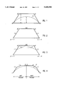
- the curve itself is described by a control polygon consisting of 4 points, p1, p2, p3, p4. Such a control polygon is shown in FIG. 1 and which also includes cubic curve 10 is being approximated.
- the dimension E is the error and defines the distance between the chord p1-p4 and the apogee of curve 10. If E is greater than ⁇ E two more polygons are constructed from the original polygon, with the property that curve 10 lies within each new polygon, and that each new polygon is the control polygon for the part of the curve which it contains. This subdivision proceeds recursively.
- the third stage involves the derivation of points l4 and r1 as follows: ##EQU3##
- the Bezier control polygons l1-l4 and r1-r4 now better approximate curve 10.
- the subdivision process ends when, any curve within a polygon is at most a distance ⁇ E from the base line of that polygon.
- the base line of the polygon is the line connecting P1 to P4).
- the calculation may be simplified by calculating the value for d instead of ⁇ E (see FIG. 1).
- Bezier subdivision generates a binary tree where each node of the tree corresponds to a subdivision step, and each edge of the tree descending from a node corresponds to a right or left control polygon that is the result of a subdivision at that node.
- the calculation cost for each node includes approximately 12 additions and 12 shifts (24 cycles).
- the error check for ⁇ E requires at least 350 additional cycles.
- most of the computational work (88%) is in computing the error condition ⁇ E at the end of each iteration. Similar disparities in calculation work exist for more complex equations, i.e., parametric quadratics, conics, etc.
- a parametric quadratic is a parametric curve whose coordinate functions are second order polynomials in the parameter t.
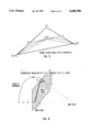
- the parametric curve is described by a triangular control polygon (see FIG. 5) consisting of three points, p 0 , p 1 , p 2 . These points define the curve as follows:
- r(p)(t) will be used to denote the curve determined by r i and l(p)(t) to denote the curve determined by l i .
- the algorithm continues recursively with each of the two output polygons being subdivided. Just as with subdivision for cubics, the subdivision process ends when the curve within the polygon is sufficiently close to the polygon, e.g., a distance less than some threshold T away.
- Bezier subdivision is applied to both the X i ,Y i and the w i to generate l(X), l(Y), l(w) and r(X), r(Y) and r(w) as in the previous section.
- the control points of the resultant curves are obtained.
- the weights of the resultant curves are the s(w) i .
- That value is determined by multiplying the total number of steps to be taken along the rotational axis times a function that results from dividing a predetermined maximum error in the number of steps to be taken along a radial axis, by the total number of steps to be taken along the radial axis for a given curve. While Ryberg's procedure is useful for curves that can be parameterized by arc length, he does not teach any method for more complex curves that do not lend themselves to such parameterization.
- a method which enables the prediction of the number of subdivisions of a curve that will be required by control polygons to assure that a resulting straight line representation of the curve will not exceed a preset error threshold.
- the method is applicable to cubics and parametric quadratics including parabolas, ellipses and hyperbolas.
- the prediction of the number of subdivisions eliminates the need for a detailed error calculation at each subdivision step, thereby enabling an error calculation to be carried out only once in the process.
- FIGS. 1-4 illustrate the prior art Bezier subdivision of a curve to enable representation of a curve by straight line segments.
- FIG. 5 illustrates a prior art Bezier subdivision of a second order curve (parabola).
- FIG. 6 illustrates a perspective projection of a 3-d parabola onto a viewplane to obtain a 2-d conic.
- FIG. 7 is a high level block diagram of a data processing system for carrying out the invention.
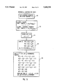
- FIG. 8 is a high level flow diagram of the method of the invention as applied to a cubic curve.
- FIG. 9 is a high level flow diagram of an alternate method of the invention as applied to a cubic curve.
- FIG. 10 is a high level flow diagram showing the application of the invention to a conic curve.
- FIG. 11 is a high level flow diagram showing a modification to the method of FIG. 10.
- FIG. 12 is a high level flow diagram showing an application of the method of the invention to an incremental algorithm for approximating a cubic curve.
- FIG. 13 is a high level flow diagram showing the application of the method to an incremental algorithm for the approximating a conic curve.
- the number of subdivisions of control polygons to simulate a curve within a certain error tolerance can be predicted by carrying out an initial error computation and then dividing the found error by a factor (e.g. the value 4) an integer number of times until the resultant error is less than a predetermined value. The number of times the error function is divided is then equal to the number of subdivisions that need to be accomplished. As a result, the required number of subdivisions is then known. This allows the required number of control polygons to be constructed, and thus gives the starting and end points of the straight lines to simulate the curve. No further error function calculations are required.
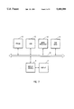
- the method of this invention can be carried out on a personal computer-sized data processing system, such as is shown in FIG. 7.
- the firmware for carrying out the method is stored in electrically programmable read only memory (EPROM) 11.
- EPROM electrically programmable read only memory
- the operation of the system is controlled by microprocessor 12 which communicates with the various elements of the system via bus 13.
- a curve's coordinate points are stored, for instance, on disk drive 14 and are transferred into random access memory (RAM) 15 when the curve approximation and display method is to be performed.
- RAM random access memory
- the algorithm takes as its input, a cubic curve specified by its control polygon (as indicated in the background of the invention and with respect to FIGS. 1-4).
- An error tolerance ⁇ E is specified and is the maximum error which the user is willing to tolerate in the curve approximation.
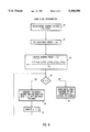
- a flow diagram illustrating the algorithm is shown. Initially, the Bezier control polygon is provided for the curve (box 20) and the maximum error ⁇ E is selected (box 22). A modified error m is then calculated by the equation shown in box 24. It will be noted that the numerator of that equation is the maximum of the second derivatives of the x and y coordinate functions at the beginning and end points of the curve. It turns out that the maximum second derivative value will always occur at either the beginning or end point of the curve, so by testing for the maximum second derivative at those points, one is able to derive the maximum second derivative coordinate function for the curve.
- the numerator result is divided by the maximum error ⁇ E and the quotient multiplied by a constant 7 ⁇ 2 to derive the modified error m.
- the constant 7 ⁇ 2 assures that the modified error m does not affect the calculation, substantially, until after approximately the second subdivision.
- the modified error m is then tested (decision box 26) to see whether its value is less than or equal to one (i.e. if the real error is less than or equal to ⁇ E ), and if it is, a line is drawn from one end of the control polygon to the other since the error limit has been reached.
- the polygon is subdivided (or if this is a subsequent step, the polygons are subdivided) leaving, for each subdivided polygon a left polygon and right polygon (box 30).
- the value of m is then divided by four and tested to determine if its new value is less than or equal to one. If not, the process repeats until the condition set in decision box 26 is met.
- the modified error calculation need only be made once, after which, the value of m is divided subsequent to a next subdivision and the effort repeated until the error condition is met.
- sufficient polygons are generated to meet the error condition without requiring additional calculations of the error function.
- Input is a Bezier cubic with its control points, and an error tolerance, ⁇ E
- log 4 (x) The value of log 4 (x) can be easily calculated by shifting.
- w 0 and w 1 are compared. It will be recalled that a rational quadratic has, for its beginning and end coordinates, three coordinate functions X, Y, and w, with w being a "weight” or third dimensional value which determines in which direction the curve is "pulled” and vice versa. If w 0 and w 1 are the beginning and end coordinate point weights, whether a curve is a hyperbola, ellipse or parabola can be determined from the following (The hyperbola modified error function is used for parabolas).
- the algorithm starts by having as its inputs, a Bezier cubic polygon specified by its coordinate functions and a specified tolerance error ⁇ E (box 50).
- the procedure then computes the value of L using the expression shown in box 52.
- the value of L is directly related to the maximum second derivative of one of the coordinate functions of the curve (L being the optimum number of step sizes required to achieve the error tolerance ⁇ E ).
- the algorithm then proceeds along the prior art incremental subdivision route shown in boxes 54, 56 and 58. In essence, the step size is chosen as being the reciprocal of 2 L .
- finite differences x t , x tt , x ttt , y t , y tt , y ttt , as defined in the Background of the invention are calculated for the x and y coordinate functions at the beginning coordinate, to a precision determined by the error tolerance and the step size. Then, the functions shown in box 58 are calculated using ⁇ t increments to determine the succeeding coordinate points.
- ⁇ t increments to determine the succeeding coordinate points.
- Dahmen's result is an estimate for the distance of the control points from the curve in terms of a constant, the granularity of the partition of the time variable, and the second derivative.
- the general form of his Theorem 2.1 gives an estimate of the form
- B i are some basis functions for the polynomial space. So, the ⁇ r i B i is an element of the polynomial space with control vector r. [Note that control points are simply coefficients in a basis. They are called control points because they also have some geometric significance]. That element is called P r . In this case, the B i are the Bernstein-Bezier (hence called B-B) Basis functions for polynomials of degree 3.
- m measures how small the sup norm of the function can get when the control points are made small.
- s n (c)(t) denote n applications of either r or l to c(t).
- s n (c)(t) is short hand for any of the curves which appear at depth n in the tree.
- s n (c) denote the particular segment at depth n which is being tested for termination. This corresponds to letting s n take on specific value.
- s 2 takes the values rl, rr, lr, and ll.
- the pointwise error after n subdivisions is
Abstract
A method enables the prediction of the number of subdivisions of a curve that will be required by control polygons to assure that a resulting straight line representation of the curve will not exceed a preset error threshold. The method is applicable to cubics and parametric quadratics including parabolas, ellipses and hyperbolas. In each case, the prediction of the number of subdivisions eliminates the need for a detailed error calculation at each subdivision step, thereby enabling an error calculation to be carried out only once in the process.
Description
This is a continuation of application Ser. No. 07/705,041, filed on May 23, 1991, now abandoned.
This invention relates to computer graphics, and more precisely, to a method and apparatus for rapidly generating curves on a computer display.
Computer graphics employ a number of techniques to reproduce curved lines and surfaces. One commonly used technique involves producing a set of points and connecting those points with straight lines to approximate the curve. The curve is successively divided into smaller pieces and then checked to see if each piece can be approximated by a straight line to within a given error threshold. It turns out that the check of the accuracy of the approximation is the dominant part of the cost of executing the curve approximation algorithm.
In a two-dimensional space, a curve is often expressed as a function of orthogonal components x and y, i.e., y is equal to f(x). In a three-dimensional coordinate system, the x, y and z coordinates may also be represented as functions of one or two of the orthogonal components. However, these representations may cause difficulty in generating the coordinate values. One alternative technique is to use a parametric representation of the curve or a representation where each coordinate value on a curve is represented as a function of some common variable, that is, a variable common to all coordinate components. For a three dimensional system, such a variable may be described as t resulting in the following: x=f(t); y=g(t); and z=h(t); for 0<t<1. A further representation is a parametric cubic curve that is represented by third order polynomials.
x=f(t)=a.sub.x t.sup.3 +b.sub.x t.sup.2 +c.sub.x t+d.sub.x
y=g(t)=a.sub.y t.sup.3 +b.sub.y t.sup.2 +c.sub.y t+d.sub.y
z=h(t)=a.sub.x t.sup.3 +b.sub.y t.sup.2 +c.sub.z t+d.sub.z
Cubic curves are important because no lower-order representation of curve segments can provide either continuity of position and slope or continuity of slope and curvature at the point where the curve segments meet. Cubic curves are also the lowest order curves that can render non-planar curves in three dimensions.
A popular prior art method for subdividing parametric cubic curves is termed "Bezier subdivision". The Bezier subdivision method will be briefly described, but no explanation or proof of its correctness will be given. Such proofs may be found in various texts on graphics, i.e., see "Fundamentals of Interactive Computer Graphic, Foley et al., Addison-Wesley Publishing Co., pp. 514-523; "Algorithms for Graphics and Image Processing", Pavlidis, Computer Science Press, pp. 220-231; and "Computational Geometry For Design and Manufacture", Faux et al., Wiley and Sons, pp. 126-145.
Given a curve and an error threshold ΔE, the Bezier algorithm produces a list of line segments which approximate the curve with errors no larger than ΔE. The curve itself is described by a control polygon consisting of 4 points, p1, p2, p3, p4. Such a control polygon is shown in FIG. 1 and which also includes cubic curve 10 is being approximated. The dimension E is the error and defines the distance between the chord p1-p4 and the apogee of curve 10. If E is greater than ΔE two more polygons are constructed from the original polygon, with the property that curve 10 lies within each new polygon, and that each new polygon is the control polygon for the part of the curve which it contains. This subdivision proceeds recursively.
An iteration of this subdivision process has three stages. The first stage is indicated in FIG. 2 wherein the following values are found: ##EQU1##
The second stage of the calculation is shown in FIG. 3 and shows the derivation of points 13 and r2 as follows: ##EQU2##
The third stage involves the derivation of points l4 and r1 as follows: ##EQU3##
At the end of the above iterations, the derived values are: ##EQU4##
As can be seen from FIG. 4, the Bezier control polygons l1-l4 and r1-r4 now better approximate curve 10. For any given resolution ΔE, the subdivision process ends when, any curve within a polygon is at most a distance ΔE from the base line of that polygon. (The base line of the polygon is the line connecting P1 to P4). The calculation may be simplified by calculating the value for d instead of ΔE (see FIG. 1).
In essence, Bezier subdivision generates a binary tree where each node of the tree corresponds to a subdivision step, and each edge of the tree descending from a node corresponds to a right or left control polygon that is the result of a subdivision at that node. In a simple implementation, the calculation cost for each node includes approximately 12 additions and 12 shifts (24 cycles). However, the error check for ΔE requires at least 350 additional cycles. Thus, most of the computational work (88%) is in computing the error condition ΔE at the end of each iteration. Similar disparities in calculation work exist for more complex equations, i.e., parametric quadratics, conics, etc.
Bezier subdivision algorithms such as the one presented for Bezier cubics exist for Bezier curves of all orders. In particular, subdivision of parametric quadratics will now be described. A parametric quadratic is a parametric curve whose coordinate functions are second order polynomials in the parameter t.
The parametric curve is described by a triangular control polygon (see FIG. 5) consisting of three points, p0, p1, p2. These points define the curve as follows:
(x(t),y(t))=p.sub.0 (1-t).sup.2 +2.sub.p 1t(1-t)+p.sub.2 t.sup.2
0<t<1
From this polygon, two more polygons are constructed with the property that half of the curve lies within each new polygon and that each new polygon is the control polygon for the part of the curve which it contains. Thus the subdivision may proceed recursively. An iteration of this subdivision process has two stages as follows: ##EQU5##
The second stage: ##EQU6## At the end of such an iteration, the values are: ##EQU7##
The notation r(p)(t) will be used to denote the curve determined by ri and l(p)(t) to denote the curve determined by li. The algorithm continues recursively with each of the two output polygons being subdivided. Just as with subdivision for cubics, the subdivision process ends when the curve within the polygon is sufficiently close to the polygon, e.g., a distance less than some threshold T away. Again, if d is the function which gives the distance from a point to a line, and l(p,q) represents the line which connects p to q, d(p1,l(p0,p2))≦T where, ##EQU8## where • is the 2-D dot product and the hat of a vector is a vector of the same length as that vector but perpendicular to it.
In this section, a prior art algorithm for drawing rational quadratics is described. It is based on using the subdivision algorithm described above to subdivide both the numerator and denominator of a rational quadratic. The control points of the subdivided numerator and denominator are divided to give the endpoints of a linear approximation to the curve.
Assume the following rational quadratic curve (x(t),y(t)) in a plane. The forms of the coordinate functions are given by: ##EQU9## Note that the numerator is expressed in the quadratic Bezier basis, as is the denominator. Henceforth, wi is required to be positive since this can be done without losing the ability to represent all rational quadratics. Geometrically, (xi, yi) are control points and wi is the weight attached to these control points. The following quantities are defined, Xi =xi wi and Yi =yi wi. These are the coordinates in the Bezier basis of the numerator, (X(t), Y(t)).
In order to draw such a curve, Bezier subdivision is applied to both the Xi,Yi and the wi to generate l(X), l(Y), l(w) and r(X), r(Y) and r(w) as in the previous section. Let s(a) denote r(a) or l(a) (i.e., "a" subdivided once). By evaluating the resultant fraction (s(X)i,s(Y)i /s(w)i, the control points of the resultant curves are obtained. The weights of the resultant curves are the s(w)i.
This is equivalent to the application of Bezier subdivision to the 3-d, second order curve (Z(t),Y(t),w(t)) followed by a perspective projection onto the x,y plane (see FIG. 6). The ending condition of the previous subsection is then applied to the curve in the x,y plane. If the subdivision is not finished, the 3-d curve is further subdivided and again projected. This continues recursively.
An Incremental Algorithms For Cubics
There are several incremental schemes for evaluating cubics. Assume a cubic curve that is specified by its two coordinate functions,
x(t)=x.sub.0 +x.sub.1 t+x.sub.2 t.sup.2 +x.sub.3 t.sup.3
y(t)=y.sub.0 +y.sub.1 t+y.sub.2 t.sup.2 +y.sub.3 t.sup.3
Suppose the values of the coordinate functions are known for some t0 and it is desired to know them for some other value t0 +Δt. Define
x.sub.t (t.sub.0)=x(t.sub.0 +Δt)-x(t.sub.0)
x.sub.tt (t.sub.0)=x.sub.t (t.sub.0 +Δt)-x.sub.t (t.sub.0)
x.sub.ttt (t.sub.0)=x.sub.tt (t.sub.0 +Δt)-x.sub.tt (t.sub.0)
y.sub.t (t.sub.0)=y(t.sub.0 +Δt)-y(t.sub.0)
y.sub.tt (t.sub.0)=y.sub.t (t.sub.0 +Δt)-y.sub.t (t.sub.0)
y.sub.ttt (t+.sub.0)=y.sub.tt (t.sub.0 +Δt)-y.sub.tt (t.sub.0)
By rewriting the above quantities in terms of the derivatives of x and y, it can be seen that xttt and yttt are constant with respect to t. Now, to get x(t+Δt) add x(t)+xt (t). To continue in this fashion, compute xt (t+Δt) in order to make the next step forward by Δt. Similarly, xtt must be updated. This leads to the following algorithm for generating points of the curve. ##EQU10##
An Incremental Algorithm for Conics
Assume a parametric quadratic coordinate function
y(t)=y.sub.0 +y.sub.1 t+y.sub.2 t.sub.2
Suppose the values of the coordinate function for some t0 are known and it is desired to know them for some other value t0 +Δt.
y.sub.t (t.sub.0)=y(t.sub.0 +Δt)-y(t.sub.0)
y.sub.tt (t.sub.0)=yt(t.sub.0 +Δt)-y.sub.t (t.sub.0)
By rewriting the above quantities in terms of the derivatives of y it can be seen that ytt is constant with respect to t. Now, to get y(t+Δt) simply add y(t)+y1 (t), continue in this fashion and compute yt (t+Δt) in order to make the next step forward by Δt. This leads to the following algorithm for generating coordinates. ##EQU11## This may be extended to an algorithm for rational quadratics in the same way the subdivision algorithm was. Namely, the above algorithm which works for a coordinate function is applied to the numerator, (X(t), Y(t)) and the denominator, w(t), and then divide to get the result.
Both prior art incremental algorithms suffer from similar problems which will be explained using cubics as an example. The incremental algorithm is more efficient than subdivision, but is also numerically ill-conditioned in the sense that errors in yttt grow cubically with the number of steps taken. That problem can be skirted, to some extent, by calculating yttt to high precision, however, precision grows cubically with the number of steps. The proper choice of value for Δt is a more difficult problem. One approach to solving this problem is adaptive subdivision which varies the size of Δt based upon the distance moved in the last step. This makes the function more expensive and more complicated.
While the Bezier subdivision technique has been described above, other derivations employ the Hermite form and the B-spline form, which forms are also considered in the above cited texts. In U.S. Pat. Nos. 4,760,548 to Baker et al, 4,912,659 to Liang 4,949,281 to Hilenbrand et al. and 4,907,282 to Daly, various aspects of B-spline curve approximation techniques are described. In U.S. Pat. Nos. 4,674,058 to Lindbloom et al. and 4,943,935 to Sato, Bezier calculations are described for curve approximation. All of the aforedescribed patents either precalculate the curve approximations and then store the results for subsequent display or calculate error values as the curves are being constructed.
In U.S. Pat. 4,855,935 to Lein, the problems inherent in recursive subdivision methods are recognized and it is suggested that a technique called "forward differencing" (advancing along a parametric curve or surface in constant parameter increments) be utilized to more efficiently generate the curve. This adaptation is performed by transforming the equation of the curve to an identical curve with different parameterization, such that the step sizes increase or decrease so that the curve proceeds in substantially uniform increments.
In U.S. Pat. No. 4,648,024 to Kato et al., curved lines (circles) instead of straight lines are employed at the lowest level of approximation for the algorithm. Other prior art concerns itself with the construction of curves that can be parameterized by arc length, i.e., a curve whose points, at equally stepped times t, are separated by a constant function or distance along the curve, (e.g. a circle). Such a system is shown in U.S. Pat. No. 4,654,805 to Shoup, II.
In U.S. Pat. No. 3,806,713 to Ryberg, a curve approximation system is described for curves having a rotational axis. Ryberg's system is based on an error in approximation of a circle by a line. Ryberg does not attempt to overcome the error calculation problem mentioned above by determining, in advance, the number of straight line segments that will be required to approximate the curve. The length of each straight line approximation is expressed by Ryberg in terms of the number of steps along the rotational axis of the curve, for each straight line approximation. That value is determined by multiplying the total number of steps to be taken along the rotational axis times a function that results from dividing a predetermined maximum error in the number of steps to be taken along a radial axis, by the total number of steps to be taken along the radial axis for a given curve. While Ryberg's procedure is useful for curves that can be parameterized by arc length, he does not teach any method for more complex curves that do not lend themselves to such parameterization.
Recently, it has been proved by Dahmen that subdivision algorithms used to reproduce curves converge in a quadratic fashion. In specific Dahmen found that the class of subdivision algorithms that includes Bezier subdivision, converges quadratically. This is equivalent to the statement that at some indeterminate point in the subdivision algorithm, the error E began to reduce in size by a factor of approximately 4 at each division step. See "Subdivision Algorithms Converge Quadratically", Dahmen, Journal of Computational and Applied Mathematics, Vol. 16, 1986, pp. 145-158. While Dahmen's results indicate that widely used subdivision algorithms do have a convergency, he does not indicate at which stage that convergency occurs and at which point in the subdivision process the error begins to be divided by a factor of 4.
Accordingly, it is an object of this invention to provide an improved method for approximating a curve through the use of straight lines, and to reduce the number of error calculations.
It is another object of this invention to provide an improved curve approximation algorithm which is particularly applicable to cubics, conics, quadratics, and other high order curvilinear equations.
A method is described which enables the prediction of the number of subdivisions of a curve that will be required by control polygons to assure that a resulting straight line representation of the curve will not exceed a preset error threshold. The method is applicable to cubics and parametric quadratics including parabolas, ellipses and hyperbolas. In each case, the prediction of the number of subdivisions eliminates the need for a detailed error calculation at each subdivision step, thereby enabling an error calculation to be carried out only once in the process.
FIGS. 1-4 illustrate the prior art Bezier subdivision of a curve to enable representation of a curve by straight line segments.
FIG. 5 illustrates a prior art Bezier subdivision of a second order curve (parabola).
FIG. 6 illustrates a perspective projection of a 3-d parabola onto a viewplane to obtain a 2-d conic.
FIG. 7 is a high level block diagram of a data processing system for carrying out the invention.
FIG. 8 is a high level flow diagram of the method of the invention as applied to a cubic curve.
FIG. 9 is a high level flow diagram of an alternate method of the invention as applied to a cubic curve.
FIG. 10 is a high level flow diagram showing the application of the invention to a conic curve.
FIG. 11 is a high level flow diagram showing a modification to the method of FIG. 10.
FIG. 12 is a high level flow diagram showing an application of the method of the invention to an incremental algorithm for approximating a cubic curve.
FIG. 13 is a high level flow diagram showing the application of the method to an incremental algorithm for the approximating a conic curve.
As indicated in the Background of the Invention, in the process of subdividing a curve into smaller segments and checking to see if each segment can be approximated by a line to within a given threshold, substantial computation time is taken up at each subdivision by the calculation of an error function. When it is realized that each subdivision creates a tree wherein the next level of subdivision doubles the number of control polygons, it can be seen that error calculations greatly hinder the curve approximation procedure. As further indicated in the Background, Dahmen has determined, theoretically, that at some point in the subdivision procedure the error decreases by a factor of four at each subsequent subdivision.
It has been found, for a curve which can be expressed as a cubic, that the reduction in error by four occurs generally after the second subdivision. Also, the largest contribution to the error function occurs as a result of attempting to simulate a complex curve with a straight line, and arises from the fact that a straight line cannot approximate the second derivative of the curve. It has been further determined that the number of subdivisions of control polygons to simulate a curve within a certain error tolerance can be predicted by carrying out an initial error computation and then dividing the found error by a factor (e.g. the value 4) an integer number of times until the resultant error is less than a predetermined value. The number of times the error function is divided is then equal to the number of subdivisions that need to be accomplished. As a result, the required number of subdivisions is then known. This allows the required number of control polygons to be constructed, and thus gives the starting and end points of the straight lines to simulate the curve. No further error function calculations are required.
The method of this invention can be carried out on a personal computer-sized data processing system, such as is shown in FIG. 7. The firmware for carrying out the method is stored in electrically programmable read only memory (EPROM) 11. The operation of the system is controlled by microprocessor 12 which communicates with the various elements of the system via bus 13. A curve's coordinate points are stored, for instance, on disk drive 14 and are transferred into random access memory (RAM) 15 when the curve approximation and display method is to be performed. Once the required number of control polygons has been determined, the coordinates of the beginning and end of each control polygon are employed by display control 16 to construct a curve approximation that is then shown on display 17.
The procedure has been found applicable to not only curves described by a cubic function, but also to rational quadratics (i.e. conics, ellipses, parabolas, and hyperbolas) and further to incremental algorithms for simulating curves. Hereafter, the algorithms for both Bezier subdivision and incremental subdivision will be described, followed by a proof section which substantiates the illustrated relationships.
The algorithm takes as its input, a cubic curve specified by its control polygon (as indicated in the background of the invention and with respect to FIGS. 1-4). An error tolerance ΔE is specified and is the maximum error which the user is willing to tolerate in the curve approximation.
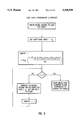
Referring to FIG. 8, a flow diagram illustrating the algorithm is shown. Initially, the Bezier control polygon is provided for the curve (box 20) and the maximum error ΔE is selected (box 22). A modified error m is then calculated by the equation shown in box 24. It will be noted that the numerator of that equation is the maximum of the second derivatives of the x and y coordinate functions at the beginning and end points of the curve. It turns out that the maximum second derivative value will always occur at either the beginning or end point of the curve, so by testing for the maximum second derivative at those points, one is able to derive the maximum second derivative coordinate function for the curve.
The numerator result is divided by the maximum error ΔE and the quotient multiplied by a constant 7√2 to derive the modified error m. The constant 7√2 assures that the modified error m does not affect the calculation, substantially, until after approximately the second subdivision. The modified error m is then tested (decision box 26) to see whether its value is less than or equal to one (i.e. if the real error is less than or equal to ΔE), and if it is, a line is drawn from one end of the control polygon to the other since the error limit has been reached. If not, the polygon is subdivided (or if this is a subsequent step, the polygons are subdivided) leaving, for each subdivided polygon a left polygon and right polygon (box 30). The value of m is then divided by four and tested to determine if its new value is less than or equal to one. If not, the process repeats until the condition set in decision box 26 is met.
It can thus be seen that the modified error calculation need only be made once, after which, the value of m is divided subsequent to a next subdivision and the effort repeated until the error condition is met. As a result, sufficient polygons are generated to meet the error condition without requiring additional calculations of the error function. In effect the number of control polygons to be used is equal to 2n, where n=the number of modified error values calculated.
The following is a pseudocode listing for the procedure shown in FIG. 8.
Input is a Bezier cubic with its control points, and an error tolerance, ΔE
Derive the second derivatives of the coordinate functions at the end of points of the cubic.
Compute the Modified Error, ##EQU12## where the primes denote differentiation. Call the subdivision routine subdivision (cubic, m)
End procedure processcubic
Begin procedure subdivision (cubic, m)
If m≦1, draw a line from one endpoint of the polygon to the other.
Otherwise,
subdivide the polygon as in the prior art, yielding two polygons, Left Polygon and Right Polygon.
call subdivision (Left Polygon, m/4)
call subdivision (Right Polygon, m/4)
end procedure subdivision
An alternative procedure (see. FIG. 9) for accomplishing the same result as above described is as follows:
Input is a Bezier cubic with its control points, and an error tolerance, ΔE
Derive the second derivatives of the coordinate functions at the end of points of the cubic.
Compute a value ##EQU13## where the primes denote differentiation. Call the subdivision routine subdivision (cubic, L)
End procedure processcubic
Begin procedure subdivision (cubic, L)
If L≦1, draw a line from one endpoint of the polygon to the other.
Otherwise,
subdivide the polygon as in the prior art, yielding two polygons, Left Polygon and Right Polygon.
call subdivision (Left Polygon, L-1)
call subdivision (Right Polygon, L-1)
end procedure subdivision
The value of log4 (x) can be easily calculated by shifting. When L=log4 (m) is computed, where m is the modified error, what is desired is that L=the smallest positive integer which is not greater than log4 (m). It is also known that m>1. So, m may be computed as follows:
if m<4, then L=1;
otherwise: L=1
while (m≧4) m=m/4; L=L+1
return (L)
This computes L by successive shifting since division by 4 is equivalent to right shifting by 2.
As will be remembered from the Background section, the coordinate functions for a rational quadratic are expressed as a fraction having quadratics in the both denominator and the numerator. If x(t), y(t) are the coordinate functions of the conic, it will be recalled (for ease of expression) that the x(t) function in the numerator and denominator, is defined as X(t)/w(t). Similarly, the expression for y(t) is simplified by letting its numerator and denominator respectively equal Y(t)/w(t). The value of ΔE is then chosen as the maximum error to be tolerated in the approximation. In the following equations, "a" can represent either x or y, as the case may be. Two quantitites are defined in terms of X, Y, w. The modified error m for an ellipse and a hyperbola (parabola) are as follows: ##EQU14##
To determine if a particular curve is an ellipse or a hyperbola, the values of w0 and w1 are compared. It will be recalled that a rational quadratic has, for its beginning and end coordinates, three coordinate functions X, Y, and w, with w being a "weight" or third dimensional value which determines in which direction the curve is "pulled" and vice versa. If w0 and w1 are the beginning and end coordinate point weights, whether a curve is a hyperbola, ellipse or parabola can be determined from the following (The hyperbola modified error function is used for parabolas).
w.sub.1 >w.sub.0 =hyperbola
w.sub.1 <w.sub.0 =ellipse
w.sub.1 =w.sub.0 =parabola.
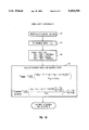
The above noted procedures are shown in boxes 40, 42, and 44 in FIG. 10.
Once the type of curve has been identified, then one or the other of the modified error equations (box 46) is solved. It will be recalled from the Background, that the Bezier polygon for a conic is an open sided triangle having points p0, p1 and p2. An equation in box 46 is thus solved by initially substituting for each "a" value the appropriate value of x. The equation is then solved. Then the appropriate values of y are inserted and the equation solved. The maximum value obtained from the solution is then equal to the modified error m for the curve.
The procedure completes by following the procedure shown in boxes 26, 28, 30, and 32 in FIG. 8. Here again, it can be seen that the number of polygonal subdivisions required to achieve the desired error is determined by the number of divisions by 4 required to reduce the value of m to less than or equal to 1.
The following is a pseudocode listing for the procedure shown in FIG. 10:
begin procedure processconic (conic, Δe)
input is a conic specified as a rational quadratic, m and an error tolerance, Δe
if the conic is an ellipse, compute m=mellipse
if the conic is an hyperbola, compute m=mhyperbola
call the conicsubdivision routine conicsubdivision (conic, m)
end procedure processconic
begin procedure conicsubdivision (conic, m)
if m≦1, draw a line from one endpoint of the conic to the other.
otherwise, subdivide the conic as in the prior art section, yielding two polygons, LeftConic and RightConic.
call conicsubdivision (LeftConic, m/4)
call conicsubdivision (RightConic, m/4) end procedure conicsubdivision
An alternative procedure (see FIG. 11) that accomplishes the same result as above is as follows:
begin procedure processconic (conic, Δe)
input is a conic specified as a rational quadratic, m and an error tolerance, Δe
if the conic is an ellipse, compute L=Log4 mellipse
if the conic is an hyperbola, compute L=Log4 mhyperbola
call the conicsubdivision routine conicsubdivision (conic, L)
end procedure processconic
begin procedure conicsubdivision (conic, m)
if L≦1, draw a line from one endpoint of the conic to the other.
otherwise, subdivide the conic as in the prior art section, yielding two polygons, LeftConic and RightConic.
call conicsubdivision (LeftConic, L-1)
call conicsubdivision (RightConic, L-1) end procedure conicsubdivision
As indicated in the Background, incremental algorithms are also used to approximate curves. Such algorithms start at one end of the curve and successively step along the curve by a predetermined amount and at each interval, determine whether the interval is small enough to give a good approximation of the curve by an inserted straight line. This invention enables the best time step along the curve to be precalculated and then simply utilized without intervening error calculations. Furthermore, rather than requiring a modified error calculation, a direct calculation is made of the optimum number of time steps to enable a given error to be achieved. It has been determined that the best number of time steps is 2L with L being dependent upon the maximum second derivative of either the x or y coordinate functions at the beginning and end points of the curve.
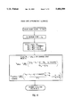
As shown in FIG. 12, the algorithm starts by having as its inputs, a Bezier cubic polygon specified by its coordinate functions and a specified tolerance error ΔE (box 50). The procedure then computes the value of L using the expression shown in box 52. Here again, the value of L is directly related to the maximum second derivative of one of the coordinate functions of the curve (L being the optimum number of step sizes required to achieve the error tolerance ΔE). The algorithm then proceeds along the prior art incremental subdivision route shown in boxes 54, 56 and 58. In essence, the step size is chosen as being the reciprocal of 2L. Next, finite differences xt, xtt, xttt, yt, ytt, yttt, as defined in the Background of the invention are calculated for the x and y coordinate functions at the beginning coordinate, to a precision determined by the error tolerance and the step size. Then, the functions shown in box 58 are calculated using Δt increments to determine the succeeding coordinate points. Here again, it is to be noted that subsequent to the calculation shown in box 52, there is no further error calculation. The requisite straight lines are then drawn.
A pseudo code description for this procedure follows:
compute ##EQU15## choose step size Δt=2-L compute x(0), xt (0), xtt (0), xttt (0) to a precision Δ E 2-L
compute y(0), yt (0), ytt (0), yttt (0) to a precision Δ E 2-L
for (t=Δt to 1, by Δt increments)
x(t)=x(t-Δt)+x.sub.t (t-Δt)
x.sub.t (t)=x.sub.t (t-Δt)+x.sub.tt (t-Δt)
x.sub.tt (t)=x.sub.tt (t-Δt)+x.sub.ttt (t-Δt)
y(t)=y(t-Δt)+y.sub.t (t-Δt)
y.sub.t (t)=y.sub.t (t-Δt)+y.sub.tt (t-Δt)
y.sub.tt (t)=y.sub.tt (t-Δt)+y.sub.ttt (t-Δt)
draw line from x(t-Δt), y(t-Δ) to x(t), y(t).
end procedure processcubic
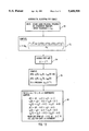
In lieu of using the Bezier subdivision for conics, an incremental subdivision technique can be employed. In this instance, the modified error expressions for both ellipses and hyperbolas are utilized, as above described. With reference to FIG. 13, a rational quadratic and error tolerance ΔE are input (box 60). Then, if the conic is determined to be an ellipse, L is computed as shown in box 62 using the modified error equation shown in box 46, FIG. 6. If, on the other hand, the conic is determined to be a hyperbola, then L is computed, as shown in box 62, using the equation shown in box 46, FIG. 6. At this point, the number of increments required to achieve an error tolerance ΔE is known. Thus, knowing the value of L, the number of steps chosen are 2L and the step size Δt is chosen as 2-L (box 64).
At this point, the procedure continues, as in prior art incremental algorithms, and computes the values shown in box 66. Subsequently, the specific increments and their weights are derived as shown in box 68, and the requisite lines drawn.
A pseudocode description for this procedure follows:
begin procedure processconic(conic, ΔE)
input is a conic specified as a rational quadratic, and an error tolerance, ΔE
if the conic is an ellipse, compute L=log4 (mellipse)
if the conic is an hyperbola, compute L=log4 (mhyperbola)
choose step size Δt=2-L
compute X(0), Xt (0), Xtt (0) to a precision Δ E 2-L
compute Y(0), Yt (0), Ytt (0) to a precision Δ E 2-L
compute w(0), wt (0), wtt (0) to a precision Δ E 2-L
for(t=Δt to 1 by Δt)
X(t)=X(t-Δt)+X.sub.t
X.sub.t (t)=X.sub.t (t-Δt)+X.sub.tt (t-Δt)
Y(t)=Y(t-Δt)+Y.sub.t (t-Δt)
Y.sub.t (t)=Y.sub.t (t-Δt)+Y.sub.tt (t-Δt)
w(t)=w(t-Δt)+w.sub.t (t-Δt)
w.sub.t (t)=w.sub.t (t-Δt)+w.sub.tt (t-Δt)
x(t)=X(t)/w(t)
y(t)=Y(t)/w(t)
draw line from x(t-Δt), y(t-Δ) to x(t), y(t)
end procedure processconic
(1) Proof of correctness of the bound for cubics
This section gives a proof of the correctness of the bound on the depth of the cursion which is necessary to make the algorithm work.
Dahmen proved [Journal of Computational and Applied Mathematics 16(1986) 145-158 "Subdivision algorithms converge quadratically"] that a class of subdivision algorithms which includes Bezier Subdivision converges quadratically and that this bound is tight in the sense that no cubic bound is possible. Using this result, along with several computations, a formula has been found for an upper bound on the depth of the tree necessary to subdivide to a given error threshold. Furthermore, this formula is readily computed (requiring 13 additions, 6 shifts, 3 compares and a variable number of shifts which is less than half the word size.) and needs to be computed only once, using quantities available before the subdivision starts.
Dahmen's result, is an estimate for the distance of the control points from the curve in terms of a constant, the granularity of the partition of the time variable, and the second derivative. The general form of his Theorem 2.1 gives an estimate of the form
|S.sub.δ -P(t.sub.δ)|<C.sub.k *δ.sup.2 *||P"||∞
Where |Sd-P(td)| is the distance between the control points and the curve, evaluated at a point which is the average of neighboring partition points. δ is a measure of the granuality of the partition, and P" is the second derivative of the curve. ||f||∞ is the L∞ norm of the function, f. k is the order of the curve. Ck is a constant which depends only on k. A special case of this result is needed where δ is a (negative) power of 2, since the subdivision can be thought of as evaluation of points on the curve for t equal to multiples of some power of 2. Due to the fact that cubics are considered, the LHS can be thought of simply as the distance from the control points to the curve. This special case result is assumed with this interpretation.
If Ck is known, then it can be found exactly how far the iteration will need to go. Dahmen's proof does not, however generate a value for Ck. The proof relies on the fact that the basis for the subdivision is uniformly stable and uses the uniform stability inequality as the starting point. In fact, a careful reading of the proof reveals that Ck is exactly the reciprocal of the constant which appears in the uniform stability inequality. So, an upper bound on Ck =m-1 is computed where ##EQU16## [Note that uniform stability of a basis is the same as m being finite and for the purposes of the proof, will be taken as the definition.] The control vector r has k+1 components and the norm on the space of control vectors is given by,
||r||=max|r.sub.i |
Bi are some basis functions for the polynomial space. So, the Σri Bi is an element of the polynomial space with control vector r. [Note that control points are simply coefficients in a basis. They are called control points because they also have some geometric significance]. That element is called Pr. In this case, the Bi are the Bernstein-Bezier (hence called B-B) Basis functions for polynomials of degree 3.
B.sub.0 (t)=(1-t).sup.3
B.sub.1 (t)=3t(2-t)
B.sub.2 (t)=3t.sup.2 (1-t)
B.sub.3 (t)=t.sup.3
So, m measures how small the sup norm of the function can get when the control points are made small. deBoor calculates the value of m for the power basis. The calculation of m for the B-B basis will follow his closely, but will have some differences which exploit features of the B-B basis. deBoor shows that an equivalent formula for m is ##EQU17## The following quantitites may be defined ##EQU18## So that m-1 =maxi mi -1 Now consider the B-B basis under the reparameterization as t goes to 1-t. This exchanges r0 with r3 and r1 with r2 but leaves the image of the curve (and hence its sup norm) unchanged. From this it can be concluded that
m.sub.0.sup.-1 =m.sub.3.sup.-1
m.sub.1.sup.-1 =m.sub.2.sup.-1
To estimate m0 -1 and m1 -1 the following fact is used together with the exact form of the transformation between the B-B basis and the power basis and the relation of the coordinates of the power basis to the derivatives. For 0≦a<b ##EQU19## where Tn-1.sup.(i) is the ith derivative of the n-1th Chebyshev polynomial, and pn is the n dimensional vector space of all polynomials of degree less than n-1. In this special case, this formula becomes ##EQU20##
Suppose a third degree polynomial, P(t). Call its coordinates in the B-B ri and its coordinates in the power basis ai, then,
r.sub.0 =a.sub.0
r.sub.1 =1/3a.sub.1 +a.sub.0
a.sub.0 =P(.sub.0)
a.sub.1 =P'(0)
It can be seen, now that m0 -1 =1 ##EQU21## The argument for m1 -1 is more involved. Pick some cubic polynomial, P, with coordinates r in the B-B basis and a in the power basis. ##EQU22## Since this inequality is valid for every polynomial in the space, it must be valid for the maximum over all polynomials in the space. ##EQU23## At the end of this calculation, the desired result is,
C.sub.3 ≦7
This may or may not be the best bound. However another calculation yields C3 ≧3.5. The difference in the upper and lower bounds is a factor of 2. Since a factor of 4 in C3 is required to double the average execution time for the algorithm there is little to gain from tightening the bound.
Now that an upper bound on C3 has been found, a calculation is needed to get the precomputable ending condition. If Dahmen's result is rewritten using the upper bound,
|S.sub.δ -P(t.sub.δ)|≦7*δ.sup.2 *||P"||∞
So, if it is required
|S.sub.δ -P(t.sub.δ)≦Δ
This can be accomplished by requiring
7*δ.sup.2 *||P"||√≦Δ
then the following is needed ##EQU24## Also, restrict d to be a power of two, say, 2-1 ##EQU25##
This reveals the error in each coordinate function, but if Euclidean error is desired another calculation is required. ##EQU26##
If the Euclidean error is bounded by ΔE, Δx and Δy must be bounded by ##EQU27## This gives a formula 1 in terms of the Euclidean error which is acceptable in the rasterized curve. ##EQU28##
Since P is assumed to be a cubic, P" is a linear function and hence must take its maximum and minimum values at the endpoints of its interval of definition. This gives ##EQU29## which is the precomputable ending condition. In the most often used special case, of ΔE =1/2, the following results
l≧log.sub.4 (max(|x"(0)|, |x"(1)|, |y"(0)|, |y"(1)|))+2.154
(2) Derivations of the ending conditions for rational quadratics (conics etc.)
This section is devoted to calculating formulae for ending conditions for conic subdivision. In para 2.2 a simple test at each iteration is shown to be an ending condition. In para 2.5 a uniform bound on the depth of subdivision necessary for a given ellipse is derived. This bound is a worst case estimate for the ending condition in 2.2. In para 2.6 a similar bound is derived for hyperbolae. In the next subsection, a bound is generated on the error in a straight line approximation to a parametric quadratic after Bezier subdivision is carried out to a depth of n. This will be used in later paragraphs to derive an ending condition and a bound on the maximum possible depth of the tree for the subdivision of rational parametric quadratics.
(2.1) Prerequisite Calculations
Consider the Bezier quadratic coordinate function
c(t)=c.sub.0 (1-t).sup.2 +2c.sub.1 t(1-t)+c.sub.2 t.sup.2
Now, consider the error made in approximating this curve for 0<t<1/2 by the line which joins c0 to c1.Also approximate c(t) by the line from c1 to c2 for 1/2<t<1. This approximation will be called approximation by the legs of the control triangle to distinguish it from approximation by the base of the control triangle which will be introduced later. The arguments for each side of 1/2 are similar and only the argument for 0<t<1/2 will be presented. In the following we will assume 0<t<1/2. The error is then,
E(c,t)=(c.sub.0 +2(c.sub.1 -c.sub.0)t)-c(t)
Take the Taylor expansion of c(t) about t=0 and calculate
E(c,t)=(2c.sub.1 -c.sub.0 c.sub.2)t.sup.2
Now, let l(c) and r(c) be the curves produced by subdividing c. The arguments for right and left side are identical, so only the left side will be shown. So, ##EQU30## Hence, with each subdivision, pointwise error is reduced by a factor of four. This is also true of the worst case error.
So, for a Curve, c(t), let sn (c)(t) denote n applications of either r or l to c(t). Hence sn (c)(t) is short hand for any of the curves which appear at depth n in the tree. In order to simplify the notation, let sn (c) denote the particular segment at depth n which is being tested for termination. This corresponds to letting sn take on specific value. For example, s2 takes the values rl, rr, lr, and ll. The pointwise error after n subdivisions is
E(s.sup.n (c), t)=(1/4).sup.n (2c.sub.1 -c.sub.0 -c.sub.2)t.sup.2
The largest absolute value of the error occurs when t=1/2 so,
max(|E(s.sup.n (c), t)|)=(1/4).sup.n+1 |2c.sub.1 -c.sub.0 -c.sub.2 |
If the curve for 0<t<1 is approximated by the line from c(0) to c(2), this is called approximation by the base of the control triangle.
By looking at a plot of c(t) and the ci in the c-t plane, it can be seen that the maximum error for approximation by the legs occur at the same point, t=1/2. This is because c(1/2) is the midpoint of the line connecting c1 with the midpoint of the line connecting c0 to c2. So, the maximum error for the two approximations is the same, occurs at the same point and the two errors are of opposite sign. From this special case, the general result can be generated.
(2.2) General Ending Condition
(2.3) Errors in the Numerator and Denominator
Recall that for the subdivision of conics, (X,Y, w) are weighted points where Xi =xi wi, Yi =yi wt which then project down under perspective projection to the correct answer. Each of these coordinate functions behaves like c of the previous paragraph. Let A denote X or Y and let a denote x or y respectively so the argument need be given only once.
The curve may be reparametrized in order to get w0 =w2. So using equation 2 it can be concluded that for approximation by the legs of the triangle,
E(s.sup.n (A), t)=(1/4).sup.n (2a.sub.1 w.sub.1 -w.sub.0 a.sub.0 -w.sub.0 a.sub.2)t.sup.2
E(s.sup.n (w), t)=(1/4).sup.n 2(w.sub.1 -w.sub.0)t.sup.2
Now, translate so that a1 lands at 0. In this new coordinate system, a0 becomes a0 -a1, a1 becomes zero, a2 becomes a2 -a1, so the error bound for sn (A)(t) becomes
E(s.sup.n (A), t)=(1/4).sup.n w.sub.0 (2a.sub.1 -a.sub.0 -a.sub.2)t.sup.2
For approximation of an ellipse by the base,
|E(s.sup.n (A), t)|≦(1/4).sup.n+1 w.sub.0 |2a.sub.1 -a.sub.0 -a.sub.2 |
0≦E(s.sup.n (w), t)≦(1/4).sup.n+1 2(w.sub.0 -w.sub.1)
recall that for an ellipse, w0 ≧w1,
(2.4) Error in a fraction
Suppose the two quantities, x+Δx and y+Δy. x and y are the true values while Δx and Δy are errors in the quantities. What is then the error in the quotient of the two quantitites. Algebra gives. ##EQU31## Applying this formula to the problem, i.e. letting x=sn (A)(t) and y=sn (w)(t), the following results ##EQU32## Dividing top and bottom by sn (w)(t) ##EQU33## By choosing approximation by the base line for ellipses and approximation by the legs for hyperbolas, it can be insured that E(sn (w),t) is non-negative. This allows the following to be written ##EQU34## By plugging in the maximum errors and taking absolute values in the numerator as well as worst case estimates for other quantities in the denominator, the following results. ##EQU35## In order to make this more computationally tractable, the fact that maxt (sn (a)(t))≦maxt (a(t)) is used and results in ##EQU36## and is precomputable before any subdivision begins. Since the control points of sn (w)(t) are known at each iteration, and are a weighted average of two quantitites, an estimate is derivable for mint (sn (w)(t)) at each iteration by using the smallest control point.
Suppose that it is wanted to ensure that E(sn (a),t)≦b. This can be done by ensuring that the right hand side of equation 4 is less than b. With rearrangement, the check for termination becomes ##EQU37## which takes one shift and one comparison at each node to compute.
Up to this point, ellipses and hyperbolas have been treated together. However, in order to prove that this is a good bound and to derive a formula to precompute the sufficient depth of a uniform tree, each case must be analyzed separately.
(2.5) Precomputable Bound for Ellipses For ellipses, it can be shown that such an estimate generates a formula for the sufficient depth of a uniform tree. This is done using the fact that for ellipses, w0 >w1 and ##EQU38## Beginning with formula 3, plugging in the bounds for ellipses, and applying the above facts, along with the fact that sn (a)(t)≦maxt (a(t)) the following results ##EQU39## If it is required that E(sn (a),t)≦b, any n satisfying ##EQU40## will do. So, for an ellipse, the ending condition will never generate a tree deeper than the bound given in the previous equation. Hence subdividing uniformly to that depth will also generate an accurate curve.
(2.6) Precomputable Bound for Hyperbolas
In this section a precomputable bound for hyperbolas is found. Starting with equation 3 and plugging in the errors for approximation by the legs, results in ##EQU41## For a hyperbola, w0 ≦w(t)≦w1 for every t. Hence, the first term in the error poses no problems, since ##EQU42## The second term, however, requires more analysis. Suppose that n is fixed and allow the meaning of s to vary. Recall that sn (w) denotes the function given by n subdivisions of w and at each subdivision, either the right or the left resultant curve may be chosen. For a hyperbola, it is clear that the choice which minimizes the absolute values of sn (w) is to choose the segment which contains one of the endpoints. Suppose the endpoint corresponding to t=0 is chosen. (The argument for t=1 is similar) Look at the quantity ##EQU43## for this segment. In particular its maximum value is to be found. A calculation shows that this quantity has nonnegative first derivatives at all points. Hence it will attain its maximum value for the maximum allowable value of t, namely 1/2. This value is ##EQU44## So with rearrangement, ##EQU45## Requiring E(sn (a),t)<b, it can be required ##EQU46## which is a precomputable depth given the curve and the error bound. Also, this is a bound on the depth to which the original error check will go since it represents a worst case for that check.
It should be understood that the foregoing description is only illustrative of the invention. Various alternatives and modifications can be devised by those skilled in the art without departing from the invention. Accordingly, the present invention is intended to embrace all such alternatives, modifications and variances which fall within the scope of the appended claims.
Claims (14)
1. A computer graphics method for approximating a curve having beginning and end coordinates by a series of connected straight line segments, said method employing a recursive subdivision of said curve and control polygons, each control polygon having at least a first straight line segment extending between two coordinates on said curve and additional connecting line segments to create a closed plane figure, a maximum distance between said first straight line segment and said curve defined as an error value, said method comprising computer implemented the steps of:
a. establishing an error value threshold ΔE between a said first straight line segment of a control polygon and said curve;
b. establishing a control polygon whose first straight line segment has terminal vertices coincident with said curve's beginning and end coordinates, calculating an error value for said control polygon and testing said error value to determine if it exceeds ΔE and if yes;
c. modifying said calculated error value by a factor and testing said modified error value to determine if it is greater than ΔE, and if it is, again modifying said modified error value by said same factor, and repeating said test, said modifying action being repeated on a last modified value until a new modified value is equal to or less than ΔE ;
d. establishing 2n control polygons between said curve's beginning and end coordinates, where n equals the number of error values calculated in steps b and c;
e. creating an approximated curve by enabling joinder of said first straight line segments of each said 2n control polygons; and
f. displaying the approximated curve on a computer display, whereby a display delay time for the step of displaying is related to an execution time for the computer graphics method.
2. The method as recited in claim 1 wherein said curve is a cubic function and said error value in step b is m which is calculated using the expression: ##EQU47## where: x" and y" are second derivatives of coordinate functions.
3. The method as recited in claim 2, wherein said modifying step includes a division of the calculated value of m by four.
4. The method as recited in claim 1 wherein said curve is a cubic function and said error value in step b is L which is calculated using the expression: ##EQU48## where: x" and y" are second derivatives of coordinate functions.
5. The method as recited in claim 4 wherein said modifying step includes the subtraction of one from L.
6. The method as recited in claim 1, wherein said curve is a conic function, said method including the additional steps of:
identifying the curve type to be one of the group: hyperbola, ellipse;
if said curve is determined to be a hyperbola, calculating a said error value for said curve in step (b) as follows: ##EQU49## if said curve is identified as an ellipse, calculating said error value for said curve in step (b) as follows: ##EQU50## where: w0, w1 are curve weight values at curve coordinates 0 and 1, respectively; t=time; and
a1, a2 are either coordinate values x1, x2 or y1, y2, as the case may be.
7. The method as recited in claim 6 wherein said modifying step includes a division of the calculated value of said error value by four.
8. The method as recited in claim 6 wherein said error value is calculated using the expression L=Log4 (m).
9. The method as recited in claim 8 wherein said modifying step includes the reduction of the value of L by one.
10. The method of claim 6 wherein said conic curve has beginning and end coordinates x(0), y(0), w(0) and x(1), y(1), w (1), and wherein step (a) identifies the curve type by the expressions
w(1)>w(0)=hyperbola
w(1)<w(0)=ellipse.
11. A computer graphics incremental method for approximating a cubic curve, having beginning and end coordinates, by a series of connected straight line segments, said method predicting the number of steps required to achieve a desired error threshold ΔE between the curve and a series of polygon line segments, wherein ΔE is a maximum distance between said curve and a line segment connecting two coordinates on said curve, each said line segment forming a portion of a polygon, said method comprising computer implemented steps of:
a) computing ##EQU51## b) choosing a step size t=2-L ; c) computing x(0), xt (0), xtt (0), xttt (0) to a precision ΔE 2-L ;
d) computing y(0), yt (0), ytt (0), yttt (0) to a precision ΔE 2-L ; and
e) for (t=Δt to 1, by Δt increments) computing:
x(t)=x(t-Δt)+x.sub.t (t-Δt),
x.sub.t (t)=x.sub.t (t-Δt)+x.sub.tt (t-Δt),
x.sub.tt (t)=x.sub.tt (t-Δt)+x.sub.ttt (t-Δt),
y(t)=y(t-Δt)+y.sub.t (t-Δt),
y.sub.t (t)=y.sub.t (t-Δt)+y.sub.tt (t-Δt),
y.sub.tt (t)=y.sub.tt (t-Δt)+y.sub.ttt (t-Δt), and
drawing a line from x(t-Δt), y(t-Δt) to x(t), y(t) for each Δt increment to create an approximated curve
where: L=number of curve subdivisions;
t=time;
x(0), y(0) are x and y coordinate functions at curve point t=0, etc.
x(0)=x coordinate function at t=0,
x.sub.t (0)=x.sub.t (t.sub.0 -Δt)-x(t.sub.0),
x.sub.tt (0)=x.sub.t (t.sub.0 +Δt)-x.sub.t (t.sub.0),
x.sub.ttt (0)=x.sub.tt (t.sub.0 +Δt) -x.sub.tt (t.sub.0),
y(0)=y coordinate function at t=0,
y.sub.t (0)=y.sub.t (t.sub.0 -Δt)-y(t.sub.0),
y.sub.tt (0)=y.sub.t (t.sub.0 +Δt)-y.sub.t (t.sub.0),
y.sub.ttt (0)=y.sub.tt (t.sub.0 +Δt) -y.sub.tt (t.sub.0), and
displaying the approximated curve on a computer display, whereby a display delay time for the step of displaying is related to an execution time for the computer graphics method.
12. A computer graphics incremental method for approximating an ellipse, having beginning and end coordinates, by a series of connected straight line segments, said method predicting the number of steps required to achieve a desired error threshold ΔE between an ellipse and a series of line segments, wherein ΔE is a maximum distance between said ellipse and a line segment connecting two coordinates on said ellipse, said method comprising computer implemented steps of:
a) computing L=log4 (mellipse) where ##EQU52## b) choosing a step size Δt=2-L c) computing X( 0), Xt (0), Xtt (0) to a precision ΔE 2-L ;
d) computing Y(0), Yt (0), Ytt (0) to a precision ΔE 2-L ;
e) computing w(0), wt (0), wtt (0) to a precision ΔE 2-L ; and
f) for (t=Δt to 1, by Δt increments) computing
X(t)=X(t-Δt)+X.sub.t (t-Δt),
X.sub.t (t)=X.sub.t (t-Δt)+X.sub.tt (t-Δt),
Y(t)=Y(t-Δt)+Y.sub.t (t-Δt),
Y.sub.t (t)=Y.sub.t (t-Δt)+Y.sub.tt (t-Δt),
w(t)-w(t-Δt)+w.sub.t (t-Δt),
w.sub.t (t)=w.sub.t (t-Δt)+w.sub.tt (t-Δt),
x(t)=X(t)/w(t),
y(t)=y(t)/w(t), and
drawing a line from x(t-Δt), y(t-Δt) to x(t), y(t) for each Δt increment to create an approximated curve
where: L=number of curve subdivisions;
w0, w1 are curve weight and values at curve coordinates 0 and 1, respectively;
t=time;
a1, a2 are either coordinate values x1, x2 or y1, y2, as the case may be;
X(0)=X(0)w(0)(at t=0);
X.sub.t (0)=X0)(t.sub.0 +Δt)-X(0)(t.sub.0);
X.sub.tt (0)=X.sub.t (0)(t.sub.0 +Δt)-X.sub.t (0)(t.sub.0);
X.sub.tt (0)=X.sub.tt (0)(t.sub.0 +Δt)-X.sub.t (0)(t.sub.0);
w(0)=weight of curve at t=0;
w.sub.t (0)=w(0)(t.sub.0 +Δt)-w(0)(t.sub.0);
w.sub.tt (0)=w.sub.t (0)(t.sub.0 +Δt)-w.sub.t (0)(t.sub.0); and
displaying the approximated curve on a computer display, whereby a display delay time for the step of displaying is related to an execution time for the computer graphics method.
13. A computer graphics incremental method for approximating a hyperbola, having beginning and end coordinates, by a series of connected straight line segments, said method predicting the number of steps L required to achieve a desired error threshold ΔE between an hyperbola and a series of line segments, wherein ΔE is a maximum distance between said hyperbola and a line segment connecting two coordinates on said hyperbola, said method comprising computer implemented steps of:
a) computing L=log4 (mhyperbola) where mhyperbola = ##EQU53## b) choosing a step size Δt=2-L c) computing X( 0), Xt (0), Xtt (0) to a precision ΔE 2-L ;
d) computing Y(0), Yt (0), Ytt (0) to a precision ΔE 2-L ;
e) computing w(0), wt (0), wtt (0) to a precision ΔE 2-L ; and
f) for (t=Δt to 1, by Δt increments) computing
X(t)=X(t-Δt)+X.sub.t (t-Δt),
x.sub.t (t)=X.sub.t (t-Δt)+X.sub.tt (t-Δt),
Y(t)=Y(t-Δt)+y.sub.t (t-Δt),
y.sub.t (t)=y.sub.t (t-Δt)+y.sub.tt (t-Δt),
w(t)=w(t-Δt)+w.sub.t (t-Δt),
w.sub.t (t)=w.sub.t (t-Δt)+w.sub.tt (t-Δt),
x(t)=X(t)/w(t),
y(t)=Y(t)/w(t), and
drawing a line from x(t-Δt), y(t-Δt) to x(t), y(t) for each Δt increment to create an approximated curve
where: L=number of curve subdivisions;
w0, w1 are curve weight and values at curve coordinates 0 and 1, respectively;
t=time;
a1, a2 are either coordinate values x1, x2 or y1, y2, as the case may be;
X(0)=X(0) w(0)(at t=0);
X.sub.t (0)=X(0)(t+Δt)-X(0)(t.sub.0);
X.sub.tt (0)=x.sub.t (0)(t.sub.0 +Δt)-X.sub.t (0)(t.sub.0);
X.sub.ttt (0)=X.sub.tt (0)(t.sub.0 +Δt)-X.sub.tt (0)(t.sub.0);
w(0)=weight of curve at t=0;
w.sub.t (0)=w(0)(t.sub.0 +Δt)-w(0)(t.sub.0);
w.sub.tt (0)=w.sub.t (0)(t.sub.0 +Δt)-w.sub.t (0)(t.sub.0); and
displaying the approximated curve on a computer display, whereby a display delay time for the step of displaying is related to an execution time for the computer graphics method.
14. A computer graphics system for approximating a curve having beginning and end coordinates by a series of connected straight line segments, said system employing a recursive subdivision procedure for said curve and control polygons to accomplish subdivision of said curve, each control polygon having at least a first straight line segment extending between two coordinates on said curve and additional connecting line segments to create a closed plane figure, a maximum distance between said first straight line segment and said curve defined as an error value, said system including a stored error value threshold ΔE, said system comprising:
means for establishing a control polygon whose first straight line segment has terminal vertices coincident with beginning and end coordinates of said curve;
means for calculating an error value for said control polygon and testing said error value to determine if it exceeds ΔE and if yes, modifying said error value that was calculated by a factor and testing said modified error value to determine if said modified error value is greater than ΔE, and if yes, again modifying said modified error value by said same factor and repeating said testing, said modifying being repeated on a last modified value by said means for calculating until a new modified value is equal to or less than ΔE ;
means for establishing 2n control polygons between said beginning and end coordinates of said curve, where n equals a number of error values calculated by said means for calculating; and
means for creating an approximated curve by joining said first straight line segments of each of said 2n control polygons and displaying the approximated curve.
Priority Applications (1)
| Application Number | Priority Date | Filing Date | Title |
|---|---|---|---|
| US08/202,678 US5408598A (en) | 1991-05-23 | 1994-02-25 | Method for fast generation of parametric curves employing a pre-calculated number of line segments in accordance with a determined error threshold |
Applications Claiming Priority (2)
| Application Number | Priority Date | Filing Date | Title |
|---|---|---|---|
| US70504191A | 1991-05-23 | 1991-05-23 | |
| US08/202,678 US5408598A (en) | 1991-05-23 | 1994-02-25 | Method for fast generation of parametric curves employing a pre-calculated number of line segments in accordance with a determined error threshold |
Related Parent Applications (1)
| Application Number | Title | Priority Date | Filing Date |
|---|---|---|---|
| US70504191A Continuation | 1991-05-23 | 1991-05-23 |
Publications (1)
| Publication Number | Publication Date |
|---|---|
| US5408598A true US5408598A (en) | 1995-04-18 |
Family
ID=24831810
Family Applications (1)
| Application Number | Title | Priority Date | Filing Date |
|---|---|---|---|
| US08/202,678 Expired - Fee Related US5408598A (en) | 1991-05-23 | 1994-02-25 | Method for fast generation of parametric curves employing a pre-calculated number of line segments in accordance with a determined error threshold |
Country Status (1)
| Country | Link |
|---|---|
| US (1) | US5408598A (en) |
Cited By (39)
| Publication number | Priority date | Publication date | Assignee | Title |
|---|---|---|---|---|
| US5500927A (en) * | 1993-03-18 | 1996-03-19 | Macromedia, Inc. | System and method for simplifying a computer-generated path |
| US5623555A (en) * | 1994-04-18 | 1997-04-22 | Lucent Technologies Inc. | Method and apparatus for handwriting decompression using estimated timing information |
| US5664071A (en) * | 1993-12-21 | 1997-09-02 | Kabushiki Kaisha Toshiba | Graphics plotting apparatus and method |
| US5790126A (en) * | 1995-01-03 | 1998-08-04 | Microsoft Corporation | Method for rendering a spline for scan conversion of a glyph |
| US5883629A (en) * | 1996-06-28 | 1999-03-16 | International Business Machines Corporation | Recursive and anisotropic method and article of manufacture for generating a balanced computer representation of an object |
| US5886703A (en) * | 1995-02-01 | 1999-03-23 | Virtus Corporation | Perspective correct texture mapping system and methods with intelligent subdivision |
| US5940083A (en) * | 1997-04-01 | 1999-08-17 | Novell, Inc. | Multi-curve rendering modification apparatus and method |
| US6115051A (en) * | 1996-08-07 | 2000-09-05 | Adobe Systems Incorporated | Arc-length reparameterization |
| US6441822B1 (en) * | 1999-04-02 | 2002-08-27 | Bruce H. Johnson | Drawing with circular arcs |
| US6614940B2 (en) * | 2001-03-09 | 2003-09-02 | Morisawa & Co., Ltd. | System, method and computer program product for generic outline font compression |
| US20050012750A1 (en) * | 2003-07-18 | 2005-01-20 | Akira Uesaki | Curved surface subdivision apparatus |
| US20060080373A1 (en) * | 2004-10-07 | 2006-04-13 | International Business Machines Corporation | Compensating for errors in performance sensitive transformations |
| US20060197759A1 (en) * | 2001-12-12 | 2006-09-07 | Technoguide As | Three dimensional geological model construction |
| US7234899B2 (en) * | 2003-05-19 | 2007-06-26 | Tdy Industries, Inc. | Cutting tool having a wiper nose corner |
| US20070189864A1 (en) * | 2003-10-15 | 2007-08-16 | Tdy Industries, Inc. | Cutting Insert for High Feed Face Milling |
| US20080170919A1 (en) * | 2007-01-16 | 2008-07-17 | Tdy Industries, Inc. | Cutting Insert, Tool Holder, and Related Method |
| US20090279962A1 (en) * | 2008-05-07 | 2009-11-12 | Tdy Industries, Inc. | Cutting tool system, cutting insert, and tool holder |
| US7627632B2 (en) | 2006-11-13 | 2009-12-01 | Microsoft Corporation | Reducing bandwidth requirements for peer-to-peer gaming based on importance of remote objects to a local player |
| US20090322916A1 (en) * | 2007-04-20 | 2009-12-31 | Sony Corporation | Signal processing system |
| US20100202839A1 (en) * | 2009-02-12 | 2010-08-12 | Tdy Industries, Inc. | Double-sided cutting inserts for high feed milling |
| US7803054B1 (en) | 2004-03-31 | 2010-09-28 | Microsoft Corporation | Multi-vehicle cross-network coordination |
| US20100272526A1 (en) * | 2009-04-28 | 2010-10-28 | Tdy Industries, Inc. | Double-sided cutting insert for drilling tool |
| US20100295858A1 (en) * | 2009-05-25 | 2010-11-25 | Fujitsu Limited | Method and system for approximating curve, and graphic display control method and apparatus |
| US20100303563A1 (en) * | 2009-02-12 | 2010-12-02 | Tdy Industries, Inc. | Double-Sided Cutting Inserts for High Feed Milling |
| US20110040797A1 (en) * | 2009-08-17 | 2011-02-17 | Tom Haskell | Geography bricks for de-identification of healthcare data |
| US20110150586A1 (en) * | 2009-12-18 | 2011-06-23 | Tdy Industries, Inc. | Tool Holder for Multiple Differently-Shaped Cutting Inserts |
| US20110148942A1 (en) * | 2009-12-22 | 2011-06-23 | Renesas Electronics Corporation | Display data correction by numerical operation suitable for display panel driver |
| US20130100138A1 (en) * | 2011-04-15 | 2013-04-25 | Takaaki Moriyama | Curve rendering device, curve rendering method, curve rendering program, and integrated circuit |
| US20130325205A1 (en) * | 2012-04-25 | 2013-12-05 | Sony Corporation | Cruise-assist image generation device, cruise-assist image generation method, in-vehicle camera and equipment-control assist image generation device |
| US8643650B1 (en) * | 2009-08-13 | 2014-02-04 | Adobe Systems Incorporated | System and method for approximating parametric curves using optimal number of segments |
| US9011049B2 (en) | 2012-09-25 | 2015-04-21 | Kennametal Inc. | Double-sided cutting inserts with anti-rotation features |
| US9283626B2 (en) | 2012-09-25 | 2016-03-15 | Kennametal Inc. | Double-sided cutting inserts with anti-rotation features |
| US9317949B2 (en) * | 2011-03-14 | 2016-04-19 | Mitsubishi Electric Corporation | String arrangement device |
| US20170200292A1 (en) * | 2016-01-12 | 2017-07-13 | Monotype Imaging Inc. | Converting Font Contour Curves |
| US20170262967A1 (en) * | 2016-03-10 | 2017-09-14 | Netflix, Inc. | Perspective correction for curved display screens |
| US10885681B2 (en) | 2015-09-11 | 2021-01-05 | Samsung Electronics Co., Ltd. | Method and apparatus for performing path stroking |
| US10936792B2 (en) | 2017-12-21 | 2021-03-02 | Monotype Imaging Inc. | Harmonizing font contours |
| CN113857789A (en) * | 2021-10-26 | 2021-12-31 | 杨官全 | Processing method of high-precision special-shaped curved surface |
| CN116705198A (en) * | 2023-03-14 | 2023-09-05 | 哈尔滨工业大学 | Liquid bridge full-range calculation method for water-soluble KDP crystal element surface microdefect DPN repair process |
Citations (14)
| Publication number | Priority date | Publication date | Assignee | Title |
|---|---|---|---|---|
| US3806713A (en) * | 1971-10-21 | 1974-04-23 | Honeywell Inf Systems | Method and apparatus for maximizing the length of straight line segments approximating a curve |
| US4648024A (en) * | 1983-11-15 | 1987-03-03 | Mitsubishi Denki Kabushiki Kaisha | Curvilinear interpolation system and method |
| US4654805A (en) * | 1985-05-06 | 1987-03-31 | Autographic Business Forms, Inc. | Computer assisted design and electromechanical operating system |
| US4674058A (en) * | 1981-12-07 | 1987-06-16 | Dicomed Corporation | Method and apparatus for flexigon representation of a two dimensional figure |
| US4760548A (en) * | 1986-06-13 | 1988-07-26 | International Business Machines Corporation | Method and apparatus for producing a curve image |
| US4855935A (en) * | 1987-05-08 | 1989-08-08 | Sun Microsystems, Inc. | Method and apparatus for rendering vectors using bresenham parameters |
| US4907282A (en) * | 1985-09-13 | 1990-03-06 | Nhance Development Corporation | Method and apparatus for constructing, storing and displaying characters |
| US4912659A (en) * | 1987-10-30 | 1990-03-27 | International Business Machines Corporation | Parallel surface processing system for graphics display |
| US4912664A (en) * | 1988-02-01 | 1990-03-27 | Mentor Graphics Corporation | Method and apparatus for generating a mesh for finite element analysis |
| US4943935A (en) * | 1987-09-25 | 1990-07-24 | Kabushiki Kaisha Toshiba | Apparatus and method for plotting curved figures represented by high order functions in a bit map |
| US4949281A (en) * | 1987-04-23 | 1990-08-14 | H. Berthold Ag | Method and apparatus for generating and producing two-dimensional graphic object by polynominal parametric curves |
| US4999789A (en) * | 1987-02-05 | 1991-03-12 | Hewlett-Packard Co. | Method and apparatus for trimming B-spline descriptions of patches in a high performance three dimensional graphics system |
| US5133052A (en) * | 1988-08-04 | 1992-07-21 | Xerox Corporation | Interactive graphical search and replace utility for computer-resident synthetic graphic image editors |
| US5214754A (en) * | 1988-06-29 | 1993-05-25 | Fujitsu Limited | Method and apparatus for approximating polygonal line to curve |
-
1994
- 1994-02-25 US US08/202,678 patent/US5408598A/en not_active Expired - Fee Related
Patent Citations (14)
| Publication number | Priority date | Publication date | Assignee | Title |
|---|---|---|---|---|
| US3806713A (en) * | 1971-10-21 | 1974-04-23 | Honeywell Inf Systems | Method and apparatus for maximizing the length of straight line segments approximating a curve |
| US4674058A (en) * | 1981-12-07 | 1987-06-16 | Dicomed Corporation | Method and apparatus for flexigon representation of a two dimensional figure |
| US4648024A (en) * | 1983-11-15 | 1987-03-03 | Mitsubishi Denki Kabushiki Kaisha | Curvilinear interpolation system and method |
| US4654805A (en) * | 1985-05-06 | 1987-03-31 | Autographic Business Forms, Inc. | Computer assisted design and electromechanical operating system |
| US4907282A (en) * | 1985-09-13 | 1990-03-06 | Nhance Development Corporation | Method and apparatus for constructing, storing and displaying characters |
| US4760548A (en) * | 1986-06-13 | 1988-07-26 | International Business Machines Corporation | Method and apparatus for producing a curve image |
| US4999789A (en) * | 1987-02-05 | 1991-03-12 | Hewlett-Packard Co. | Method and apparatus for trimming B-spline descriptions of patches in a high performance three dimensional graphics system |
| US4949281A (en) * | 1987-04-23 | 1990-08-14 | H. Berthold Ag | Method and apparatus for generating and producing two-dimensional graphic object by polynominal parametric curves |
| US4855935A (en) * | 1987-05-08 | 1989-08-08 | Sun Microsystems, Inc. | Method and apparatus for rendering vectors using bresenham parameters |
| US4943935A (en) * | 1987-09-25 | 1990-07-24 | Kabushiki Kaisha Toshiba | Apparatus and method for plotting curved figures represented by high order functions in a bit map |
| US4912659A (en) * | 1987-10-30 | 1990-03-27 | International Business Machines Corporation | Parallel surface processing system for graphics display |
| US4912664A (en) * | 1988-02-01 | 1990-03-27 | Mentor Graphics Corporation | Method and apparatus for generating a mesh for finite element analysis |
| US5214754A (en) * | 1988-06-29 | 1993-05-25 | Fujitsu Limited | Method and apparatus for approximating polygonal line to curve |
| US5133052A (en) * | 1988-08-04 | 1992-07-21 | Xerox Corporation | Interactive graphical search and replace utility for computer-resident synthetic graphic image editors |
Non-Patent Citations (6)
| Title |
|---|
| Computer Science Press, Inc., "Algorithms for Graphics and Image Processing", Theo Pavlidis Bell Laboratories, pp. 221-231., 1982. |
| Computer Science Press, Inc., Algorithms for Graphics and Image Processing , Theo Pavlidis Bell Laboratories, pp. 221 231., 1982. * |
| I. D. Faux et al., "Computational Geometry for Design and Manufacture", Dept. of Mathematics 1979, pp. 127-145. Publisher: E. Horwood Ltd. |
| I. D. Faux et al., Computational Geometry for Design and Manufacture , Dept. of Mathematics 1979, pp. 127 145. Publisher: E. Horwood Ltd. * |
| Wolfgang Dahmen, "Subdivision Algorithms Converge Quadratically", 1988, pp. 145-158, Journal of Computational and Applied Mathimatics. |
| Wolfgang Dahmen, Subdivision Algorithms Converge Quadratically , 1988, pp. 145 158, Journal of Computational and Applied Mathimatics. * |
Cited By (80)
| Publication number | Priority date | Publication date | Assignee | Title |
|---|---|---|---|---|
| US5500927A (en) * | 1993-03-18 | 1996-03-19 | Macromedia, Inc. | System and method for simplifying a computer-generated path |
| US5664071A (en) * | 1993-12-21 | 1997-09-02 | Kabushiki Kaisha Toshiba | Graphics plotting apparatus and method |
| US5623555A (en) * | 1994-04-18 | 1997-04-22 | Lucent Technologies Inc. | Method and apparatus for handwriting decompression using estimated timing information |
| US6088041A (en) * | 1995-01-03 | 2000-07-11 | Microsoft Corporation | Method of dropout control for scan conversion of a glyph comprising a plurality of discrete segments |
| US6529197B1 (en) | 1995-01-03 | 2003-03-04 | Microsoft Corporation | Method for rendering endpoints of segments during scan conversion of a glyph |
| US5867173A (en) * | 1995-01-03 | 1999-02-02 | Microsoft Corporation | Method for rendering a spline for scan conversion of a glyph comprising a plurality of discrete segments |
| US5790126A (en) * | 1995-01-03 | 1998-08-04 | Microsoft Corporation | Method for rendering a spline for scan conversion of a glyph |
| US6175372B1 (en) | 1995-01-03 | 2001-01-16 | Dean Dayton Ballard | Method for estimating the memory required for scan conversation of a glyph |
| US5886703A (en) * | 1995-02-01 | 1999-03-23 | Virtus Corporation | Perspective correct texture mapping system and methods with intelligent subdivision |
| US5883629A (en) * | 1996-06-28 | 1999-03-16 | International Business Machines Corporation | Recursive and anisotropic method and article of manufacture for generating a balanced computer representation of an object |
| US6115051A (en) * | 1996-08-07 | 2000-09-05 | Adobe Systems Incorporated | Arc-length reparameterization |
| US5940083A (en) * | 1997-04-01 | 1999-08-17 | Novell, Inc. | Multi-curve rendering modification apparatus and method |
| US6441822B1 (en) * | 1999-04-02 | 2002-08-27 | Bruce H. Johnson | Drawing with circular arcs |
| US6614940B2 (en) * | 2001-03-09 | 2003-09-02 | Morisawa & Co., Ltd. | System, method and computer program product for generic outline font compression |
| US7542037B2 (en) * | 2001-12-12 | 2009-06-02 | Schlumberger Technology Corporation | Three dimensional geological model construction |
| US20060197759A1 (en) * | 2001-12-12 | 2006-09-07 | Technoguide As | Three dimensional geological model construction |
| US7234899B2 (en) * | 2003-05-19 | 2007-06-26 | Tdy Industries, Inc. | Cutting tool having a wiper nose corner |
| US20050012750A1 (en) * | 2003-07-18 | 2005-01-20 | Akira Uesaki | Curved surface subdivision apparatus |
| US7015917B2 (en) * | 2003-07-18 | 2006-03-21 | Matsushita Electric Industrial Co., Ltd. | Curved surface subdivision apparatus |
| US7600952B2 (en) | 2003-10-15 | 2009-10-13 | Tdy Industries, Inc. | Cutting insert for high feed face milling |
| US8162572B2 (en) | 2003-10-15 | 2012-04-24 | TDY Industries, LLC | Cutting insert for high feed face milling |
| US20100284753A1 (en) * | 2003-10-15 | 2010-11-11 | Tdy Industries, Inc. | Cutting Insert for High Feed Face Milling |
| US20090097929A1 (en) * | 2003-10-15 | 2009-04-16 | Tdy Industries, Inc. | Cutting insert for high feed face milling, and milling cutter tool including same |
| US20070189864A1 (en) * | 2003-10-15 | 2007-08-16 | Tdy Industries, Inc. | Cutting Insert for High Feed Face Milling |
| US7988387B2 (en) | 2003-10-15 | 2011-08-02 | Tdy Industries, Inc. | Cutting insert for high feed face milling |
| US8821080B2 (en) | 2003-10-15 | 2014-09-02 | Kennametal Inc. | Cutting insert for high feed face milling |
| US7806634B2 (en) | 2003-10-15 | 2010-10-05 | Tdy Industries, Inc. | Cutting insert for high feed face milling, and milling cutter tool including same |
| US8444352B2 (en) | 2003-10-15 | 2013-05-21 | TDY Industries, LLC | Cutting insert for high feed face milling |
| US9446460B2 (en) | 2003-10-15 | 2016-09-20 | Kennametal Inc. | Cutting insert for high feed face milling |
| US7803054B1 (en) | 2004-03-31 | 2010-09-28 | Microsoft Corporation | Multi-vehicle cross-network coordination |
| US20060080373A1 (en) * | 2004-10-07 | 2006-04-13 | International Business Machines Corporation | Compensating for errors in performance sensitive transformations |
| US7489826B2 (en) * | 2004-10-07 | 2009-02-10 | Infoprint Solutions Company, Llc | Compensating for errors in performance sensitive transformations |
| US20100035695A1 (en) * | 2006-11-13 | 2010-02-11 | Microsoft Corporation | Reducing bandwidth requirements for peer-to-peer gaming based on importance of remote objects to a local player |
| US7627632B2 (en) | 2006-11-13 | 2009-12-01 | Microsoft Corporation | Reducing bandwidth requirements for peer-to-peer gaming based on importance of remote objects to a local player |
| US7925601B2 (en) | 2006-11-13 | 2011-04-12 | Microsoft Corporation | Reducing bandwidth requirements for peer-to-peer gaming based on error difference between actual game object state and simulated game object state being below an error threshold |
| US7905687B2 (en) | 2007-01-16 | 2011-03-15 | Tdy Industries, Inc. | Cutting insert, tool holder, and related method |
| US20080170919A1 (en) * | 2007-01-16 | 2008-07-17 | Tdy Industries, Inc. | Cutting Insert, Tool Holder, and Related Method |
| US7852380B2 (en) | 2007-04-20 | 2010-12-14 | Sony Corporation | Signal processing system and method of operation for nonlinear signal processing |
| US20090322916A1 (en) * | 2007-04-20 | 2009-12-31 | Sony Corporation | Signal processing system |
| US20090279962A1 (en) * | 2008-05-07 | 2009-11-12 | Tdy Industries, Inc. | Cutting tool system, cutting insert, and tool holder |
| US7905689B2 (en) | 2008-05-07 | 2011-03-15 | Tdy Industries, Inc. | Cutting tool system, cutting insert, and tool holder |
| US7976250B2 (en) | 2009-02-12 | 2011-07-12 | Tdy Industries, Inc. | Double-sided cutting inserts for high feed milling |
| US20100202839A1 (en) * | 2009-02-12 | 2010-08-12 | Tdy Industries, Inc. | Double-sided cutting inserts for high feed milling |
| US20100303563A1 (en) * | 2009-02-12 | 2010-12-02 | Tdy Industries, Inc. | Double-Sided Cutting Inserts for High Feed Milling |
| US8491234B2 (en) | 2009-02-12 | 2013-07-23 | TDY Industries, LLC | Double-sided cutting inserts for high feed milling |
| US20100272526A1 (en) * | 2009-04-28 | 2010-10-28 | Tdy Industries, Inc. | Double-sided cutting insert for drilling tool |
| US9586264B2 (en) | 2009-04-28 | 2017-03-07 | Kennametal Inc. | Double-sided cutting insert for drilling tool |
| US20100295858A1 (en) * | 2009-05-25 | 2010-11-25 | Fujitsu Limited | Method and system for approximating curve, and graphic display control method and apparatus |
| CN101901488B (en) * | 2009-05-25 | 2015-09-09 | 富士通株式会社 | For the method and apparatus of curve approximation and figure display control method and device |
| US8976183B2 (en) | 2009-05-25 | 2015-03-10 | Fujitsu Limited | Method and system for approximating curve, and graphic display control method and apparatus |
| EP2256692A1 (en) * | 2009-05-25 | 2010-12-01 | Fujitsu Limited | Method and system for approximating a curve for display purposes, and graphic display control method and apparatus |
| US8643650B1 (en) * | 2009-08-13 | 2014-02-04 | Adobe Systems Incorporated | System and method for approximating parametric curves using optimal number of segments |
| US8296299B2 (en) * | 2009-08-17 | 2012-10-23 | Ims Software Services Ltd. | Geography bricks for de-identification of healthcare data |
| US20110040797A1 (en) * | 2009-08-17 | 2011-02-17 | Tom Haskell | Geography bricks for de-identification of healthcare data |
| US8807884B2 (en) | 2009-12-18 | 2014-08-19 | Kennametal Inc. | Tool holder for multiple differently-shaped cutting inserts |
| US20110150586A1 (en) * | 2009-12-18 | 2011-06-23 | Tdy Industries, Inc. | Tool Holder for Multiple Differently-Shaped Cutting Inserts |
| US10672360B2 (en) * | 2009-12-22 | 2020-06-02 | Renesas Electronics Corporation | Display data correction by numerical operation suitable for display panel driver |
| US20110148942A1 (en) * | 2009-12-22 | 2011-06-23 | Renesas Electronics Corporation | Display data correction by numerical operation suitable for display panel driver |
| US9317949B2 (en) * | 2011-03-14 | 2016-04-19 | Mitsubishi Electric Corporation | String arrangement device |
| US20130100138A1 (en) * | 2011-04-15 | 2013-04-25 | Takaaki Moriyama | Curve rendering device, curve rendering method, curve rendering program, and integrated circuit |
| US9092905B2 (en) * | 2011-04-15 | 2015-07-28 | Panasonic Intellectual Property Management Co., Ltd. | Curve rendering device, curve rendering method, curve rendering program, and integrated circuit |
| US20130325205A1 (en) * | 2012-04-25 | 2013-12-05 | Sony Corporation | Cruise-assist image generation device, cruise-assist image generation method, in-vehicle camera and equipment-control assist image generation device |
| US11628882B2 (en) | 2012-04-25 | 2023-04-18 | Sony Group Corporation | Cruise-assist image generation device, cruise-assist image generation method, in-vehicle camera and equipment-control assist image generation device |
| US9533709B2 (en) * | 2012-04-25 | 2017-01-03 | Sony Corporation | Cruise-assist image generation device, cruise-assist image generation method, in-vehicle camera and equipment-control assist image generation device |
| US10696328B2 (en) | 2012-04-25 | 2020-06-30 | Sony Corporation | Cruise-assist image generation device, cruise-assist image generation method, in-vehicle camera and equipment-control assist image generation device |
| US9283626B2 (en) | 2012-09-25 | 2016-03-15 | Kennametal Inc. | Double-sided cutting inserts with anti-rotation features |
| US9011049B2 (en) | 2012-09-25 | 2015-04-21 | Kennametal Inc. | Double-sided cutting inserts with anti-rotation features |
| US10885681B2 (en) | 2015-09-11 | 2021-01-05 | Samsung Electronics Co., Ltd. | Method and apparatus for performing path stroking |
| US20170200292A1 (en) * | 2016-01-12 | 2017-07-13 | Monotype Imaging Inc. | Converting Font Contour Curves |
| US10347016B2 (en) * | 2016-01-12 | 2019-07-09 | Monotype Imaging Inc. | Converting font contour curves |
| US10366476B2 (en) * | 2016-03-10 | 2019-07-30 | Netflix, Inc. | Perspective correction for curved display screens |
| US20170262967A1 (en) * | 2016-03-10 | 2017-09-14 | Netflix, Inc. | Perspective correction for curved display screens |
| US9792674B2 (en) * | 2016-03-10 | 2017-10-17 | Netflix, Inc. | Perspective correction for curved display screens |
| CN109074773B (en) * | 2016-03-10 | 2021-12-07 | 奈飞公司 | Perspective correction for curved display screens |
| CN109074773A (en) * | 2016-03-10 | 2018-12-21 | 奈飞公司 | For the perspective correction of flexible displays screen |
| US10936792B2 (en) | 2017-12-21 | 2021-03-02 | Monotype Imaging Inc. | Harmonizing font contours |
| CN113857789A (en) * | 2021-10-26 | 2021-12-31 | 杨官全 | Processing method of high-precision special-shaped curved surface |
| CN113857789B (en) * | 2021-10-26 | 2024-03-22 | 杨官全 | Processing method of high-precision special-shaped curved surface |
| CN116705198A (en) * | 2023-03-14 | 2023-09-05 | 哈尔滨工业大学 | Liquid bridge full-range calculation method for water-soluble KDP crystal element surface microdefect DPN repair process |
| CN116705198B (en) * | 2023-03-14 | 2023-11-17 | 哈尔滨工业大学 | Liquid bridge full-range calculation method for water-soluble KDP crystal element surface microdefect DPN repair process |
Similar Documents
| Publication | Publication Date | Title |
|---|---|---|
| US5408598A (en) | Method for fast generation of parametric curves employing a pre-calculated number of line segments in accordance with a determined error threshold | |
| US5367617A (en) | System and method of hybrid forward differencing to render Bezier splines | |
| Lancaster et al. | Surfaces generated by moving least squares methods | |
| US5278948A (en) | Parametric surface evaluation method and apparatus for a computer graphics display system | |
| Kopriva et al. | A conservative staggered-grid Chebyshev multidomain method for compressible flows | |
| US5636338A (en) | Method for designing curved shapes for use by a computer | |
| US6211883B1 (en) | Patch-flatness test unit for high order rational surface patch rendering systems | |
| JP3318914B2 (en) | System and method for rendering Bezier splines | |
| US5317682A (en) | Parametric curve evaluation method and apparatus for a computer graphics display system | |
| Gonzalez et al. | High-order parameterization of stable/unstable manifolds for long periodic orbits of maps | |
| Bertolazzi et al. | Point data reconstruction and smoothing using cubic splines and clusterization | |
| Xie et al. | Automatic knot determination of NURBS for interactive geometric design | |
| Kumar et al. | Parameter optimization for B-spline curve fitting using genetic algorithms | |
| US6226405B1 (en) | Method and apparatus for updating node position | |
| EP0349182B1 (en) | Method and apparatus for approximating polygonal line to curve | |
| Fletcher et al. | Automatic tension adjustment for interpolatory splines | |
| Korostyshevskiy et al. | A Hermite spectral method for the computation of homoclinic orbits and associated functionals | |
| JP4175470B2 (en) | CAD system, curved surface analyzing apparatus, curved surface reproducing apparatus, method and program thereof | |
| Van Barel et al. | Orthogonal rational functions and diagonal-plus-semiseparable matrices | |
| Kersey | On the problems of smoothing and near-interpolation | |
| McFadden | Lectures on simulation-assisted statistical inference | |
| Farin | Shape | |
| Triggs | Some notes on factorization methods for projective structure and motion | |
| Han et al. | Representing multifigure anatomical objects | |
| Asteasu et al. | Parametric piecewise surfaces intersection |
Legal Events
| Date | Code | Title | Description |
|---|---|---|---|
| CC | Certificate of correction | ||
| REMI | Maintenance fee reminder mailed | ||
| LAPS | Lapse for failure to pay maintenance fees | ||
| FP | Lapsed due to failure to pay maintenance fee |
Effective date: 19990418 |
|
| STCH | Information on status: patent discontinuation |
Free format text: PATENT EXPIRED DUE TO NONPAYMENT OF MAINTENANCE FEES UNDER 37 CFR 1.362 |