US8943113B2 - Methods and systems for parsing and interpretation of mathematical statements - Google Patents
Methods and systems for parsing and interpretation of mathematical statements Download PDFInfo
- Publication number
- US8943113B2 US8943113B2 US13/188,090 US201113188090A US8943113B2 US 8943113 B2 US8943113 B2 US 8943113B2 US 201113188090 A US201113188090 A US 201113188090A US 8943113 B2 US8943113 B2 US 8943113B2
- Authority
- US
- United States
- Prior art keywords
- mathematical
- instruction
- statements
- expressions
- dimensional
- Prior art date
- Legal status (The legal status is an assumption and is not a legal conclusion. Google has not performed a legal analysis and makes no representation as to the accuracy of the status listed.)
- Expired - Fee Related, expires
Links
Images
Classifications
-
- G06F17/215—
-
- G—PHYSICS
- G06—COMPUTING; CALCULATING OR COUNTING
- G06F—ELECTRIC DIGITAL DATA PROCESSING
- G06F40/00—Handling natural language data
- G06F40/10—Text processing
- G06F40/103—Formatting, i.e. changing of presentation of documents
- G06F40/111—Mathematical or scientific formatting; Subscripts; Superscripts
Definitions
- the following relates generally to mathematical statement recognition and evaluation and more specifically to methods and systems for recognition and evaluation of hybrid statements mixing symbolic expressions and natural language including English provided in one-dimensional formats using ASCII.
- Math software has been developed to perform symbolic and/or numerical mathematical computations that have been otherwise performed by humans. For educational users, such as advanced junior high school students, high school students and college students, math software tools may be used to assist in the learning process. Math software can provide efficient results for what are often time consuming and tedious tasks if performed manually. Once a student has an understanding of a process or calculation, using that process or calculation as a building block in other, perhaps more complex, calculations or processes is an important task. However, the time consuming nature of performing such a task may hinder the amount of tasks that such a student may accomplish. Thus, efficient software tools may assist in the educational process by reducing the amount of such tasks. Furthermore, such software may provide encouragement for the learning of different processes and concepts.
- a computer language is required to convert a math problem defined in natural mathematics language, which includes symbolic expressions in natural math notations, and hybrid statements mixing natural language and symbolic expressions for defining operations applicable to and relationships among mathematical entities, into an intermediate representation such as abstract syntax tree (AST) that can invoke appropriate algorithms written in, for example, other lower level languages such as C or Fortran that perform the defined mathematical computations.
- AST abstract syntax tree
- Item A causes many users to spend a long time learning to use the software, creating a significant barrier to use and consequently impeding market acceptance. The impact is even worse for student users: instead of assisting, the software/devices actually complicate a student's learning because he or she is forced to navigate simultaneously two different sets of notations, one from a textbook and another for the software.
- Item B makes it difficult for many users to define math problems since the expressive power of symbolic expressions is nevertheless limited beyond imperatives. Consequently, users have to decompose these problems and write procedural code to solve the problems using primitive constructs provided by the language. This is obviously not plausible for most students learning math or professional users that are not programming-savvy. In fact, it defies the purpose of mathematically-oriented languages and software. For instance, any individual able to write detailed procedural code to solve a math problem is less likely to need the help of math software in the first place.
- the present disclosure generally relates to one or more improved systems, methods, and/or apparatuses for parsing and interpretation of mathematical statements, including what are referred to as hybrid mathematical statements that combine mathematical notation and natural language.
- Embodiments disclosed herein provide a rigorous and practically tractable formal grammar to distill the essence of the following:
- the disclosure herein also provides a unique work flow for receiving and processing one or more statements.
- the work flow comprises (a) an input step for receiving at least one one-dimensional statement from a user; (b) a parsing procedure, utilizing a grammar library, that operates on the received statement(s) to convert the one-dimensional statement(s) into one or more intermediate representation such as an abstract syntax tree (AST) representing mathematical expressions and the manipulations imposed on them; and (c) an interpretation procedure that evaluates the mathematical expressions embedded in the ASTs and executes the manipulations in accordance with the AST, and provides a result.
- AST abstract syntax tree
- both the result as well as narratives similar to human-constructed solutions are provided, in a format ready for display in natural mathematical notation.
- compositions provide methodologies that enable the composition of step-by-step procedures and narratives explaining the concepts and background involved in solving math problems, for a math software that employs the above-mentioned computer language.
- the composition is similar to human-made solutions and thus easy to follow for users such as students.
- a further aspect of the disclosure provides a computer program product comprising a non-transitory computer readable medium comprising: (a) code for receiving one or more one-dimensional hybrid statements mixing mathematical expressions and natural language; (b) code for converting, via at least one call to a grammar library, portions of the one or more one-dimensional hybrid statements into a plurality of mathematical expressions and one or more abstract syntax tree (AST) of the expressions, wherein the grammar library includes rules for performing the step of converting; (c) code for initially displaying a two dimensional mathematical expression representing the one or more hybrid mathematical expressions; (d) code for evaluating the mathematical expressions in accordance with the AST of the expressions; and (e) code for displaying a two dimensional mathematical expression representing a narrative for the evaluation of the mathematical expressions.
- novel functionality for method for receiving and evaluating a hybrid mathematical statement, comprising: (a) receiving one or more one-dimensional hybrid statements mixing mathematical expressions and natural language; (b) converting, via at least one call to a grammar library, portions of one or more one-dimensional hybrid statements into a plurality of one or more abstract syntax tree (AST) of the expressions, wherein the grammar library includes rules for performing the step of converting; (c) evaluating the hybrid statements in accordance with the AST; and (d) performing at least one of storing and transmitting a result of the evaluation.
- AST abstract syntax tree
- FIG. 1 is a flowchart of a method for receiving and evaluating hybrid mathematical statements according to an exemplary embodiment
- FIG. 2 is a flowchart of a method for receiving and evaluating hybrid mathematical statements according to another exemplary embodiment
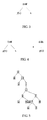
- FIG. 3 illustrates an exemplary hierarchical structure of traditional operator for derivatives as a binary operator
- FIG. 4 illustrates an exemplary transformation of traditional operator for derivatives into an unary operator with variable being differentiated absorbed by the operator
- FIG. 5 illustrates an exemplary hierarchical structure of set definition through set-builder notation
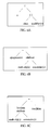
- FIGS. 6A-6C illustrate exemplary hierarchical structures of assertion statements
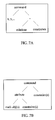
- FIGS. 7A-7B illustrate exemplary hierarchical structures of command statements
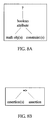
- FIG. 8A illustrates an exemplary hierarchical structure of a query statement according to an embodiment
- FIG. 8B illustrates an exemplary hierarchical structure of deduction statement according to an embodiment
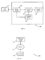
- FIG. 9 illustrates a block diagram of an exemplary system according to an embodiment
- FIG. 10 shows a block diagram of an exemplary system according to another embodiment
- FIGS. 11A-11B are screen shots captured after exemplary one-dimensional mathematical statements are entered according to an exemplary embodiment.
- FIGS. 12A-12C are screen shots captured after exemplary one-dimensional mathematical statements are entered and interpreted according to an exemplary embodiment.
- math notation is 2-dimensional in that it uses both symbols as well as vertical positioning such as overhead and superscript to convey semantics.
- ASCII the character set that commonly used for communication between human and computing software/devices is 1-dimensional in the sense that characters are aligned horizontally when entered;
- the natural math notation employs many symbols including Greek letters and specially-created symbols such as and E that are not included in ASCII; and
- the syntaxes of math notation can be context-sensitive. This combination presents a serious challenge to the development of a formal grammar that abstracts the syntactical structures, which is the core of a language usable by the software and devices.
- the present disclosure provides a mathematical notation friendly language defined by a rigorous yet practically tractable formal grammar to make the one-dimension representation of mathematical expressions either appears physically similar, or is easily associable to, their forms in natural math notation.
- a variety of methods including leveling, asciilization, direct adoption and operator transformation to minimize the syntactical gap between the language and the math notation.
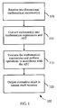
- one or more one-dimensional mathematical statements are received, according to block 105 .
- the one-dimensional statements include one or more hybrid statements mixing mathematical expressions and natural language.
- a user may enter one or more one-dimensional statements into a system using a keyboard to enter ACSII text in multiple input lines that represent one or more mathematical statements.
- the statements are then converted into one or more abstract syntax tree (AST), at block 110 .
- AST abstract syntax tree
- One-dimensional statements, including hybrid statements, and conversion of such statements will be described in more detail below.
- the mathematical statements are interpreted in accordance with the AST, at block 115 .
- the results are displayed in natural math notation, according to block 120 .
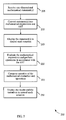
- a user may enter one or more one-dimensional statements into a system using a keyboard, for example.
- the statements are then converted into one or more AST, at block 210 .
- Mathematical statements, including hybrid statements, and conversion of such statements will be described in more detail below.
- two-dimensional representations for the statements in natural math notation are displayed.
- a user may be prompted to verify that the displayed expression corresponds to what the user intended.
- the mathematical statements are interpreted and mathematical operations are performed in accordance with the AST, at block 220 .
- Narratives are composed accompanying the interpretation of statements according to block 225 .
- the results of the interpretation and narratives are displayed in natural math notation, according to block 230 . Again, the display of step-by-step problem solving narratives may assist a user in understanding various mathematical concepts.
- mathematical notation is often two-dimensional in nature, since it not only relies on symbols themselves but also their relative positions (superscript, subscript, overhead, etc.) to convey semantics
- default computer code written in ASCII set is one-dimensional, i.e., all characters are aligned horizontally, which can provide an obstacle to providing a user friendly and highly functional mathematical application in situations where it is more convenient for a user to enter information using ASCII characters.
- math notation routinely employs many characters such as Greek letters for variables and constants ( ⁇ for example), and some of the letters are given special meanings. For example, ⁇ is used for summation and ⁇ is used for product.
- Math notation also employs symbols particularly designed for mathematics, such as ⁇ for integration, ⁇ for partial differentiation, and ⁇ for gradient operator for vector field. Furthermore, even if input were available to accommodate all sorts of math symbols that are not included in ASCII, and templates for all sorts of position-dependent structures (power, limit, integration, etc.), a formal grammar would be needed in order to capture the rich syntaxes of mathematical language.
- the syntaxes of mathematical language are far more complicated then what present day computer languages are capable of expressing directly, whose expressive capacity is usually limited to arithmetic operations ( ⁇ , ⁇ , ⁇ ) and common control structures (loop, if/else construct, etc).
- the present disclosure provides that mathematical expressions be input through ASCII characters, and no other character set such as Unicode is included as an input option in various embodiments.
- This constraint requires that the aforementioned three obstacles be explicitly taken into consideration.
- the approaches and syntaxes used to solve these problems include several novel features. Exemplary methods employed include leveling, asciilization, and adoption and operator transformation.
- the leveling technique refers to the transformation that makes two-dimensional math structures one-dimensional by placing superscript, subscript and overhead symbols that decorate another symbol to normal positions in manner that is intuitive for users to form a connection to the corresponding natural math notation.
- leveling is the expression for definite integral. It is two dimensional due to the existence of upper and lower bound defining the integral.
- the bound can be expressed using a notation for range, “a ⁇ x ⁇ b”. Additionally, rules are required for where to place such a range and how to link to the indefinite integral.
- the expression “$f(x)dx” is used to express an integration function. Exemplary expressions are included below in Table 1. With respect to the range notation, this can be placed after the integration sign or at the end of the definition of the indefinite integral. In one embodiment, this statement is placed after the indefinite integral, and the symbol “@” is introduced to separate the indefinite integral and the integration domain.
- Leveling techniques has also been used to represent family of what we called postfix unary operators that are formed by placing operator symbols after the symbol ⁇ indicating the operator is positioned on the shoulder or above the operand, such as ⁇ (vector normalization), ⁇ . and ⁇ .. (Newton's notation), ⁇ ′, ⁇ ′′ and f ⁇ (n) for Lagrange's notation.
- ⁇ vector normalization
- ⁇ . and ⁇ .. Newton's notation
- ⁇ ′, ⁇ ′′ and f ⁇ (n) for Lagrange's notation.
- a favorable side-effect of having a dedicated representation for the Lagrange notation is that x′ can be used for a variable loosely related to x, which can be useful for applications such as coordinate transformations and those involving Green's functions.
- the treatments for limit, summation and product are similar, as shown in Table 1.
- ⁇ - is a postfix unary operator that means less than but infinitely close to a variable when placed after that operator. That is very convenient in expressing a fundamental concept in calculus, namely the limit: lim( f ( x ))@( x ⁇ >a ⁇ -)
- f ⁇ (n)(x) means the n th -order derivative of f(x)w.r.t.x when n ⁇ 1;
- f ⁇ n(x) means the n-th power of f ⁇ (x) with f ⁇ 1(x) being reserved for the inverse of f, where f is a function.
- the ascillization technique is used to decrease the difference between the computer language and natural math notation associated with the lack of special characters/symbols.
- embodiments simply use ASCII characters or strings to represent the special symbols through some sort of connection.
- One type of connection is through phonetics.
- the representations of Greek letters are based on this connection.
- Another connection is based on visual or calligraphic similarity. Examples include using $ to represent elongated-s symbol ⁇ for integration, and ⁇ to represent belong-to symbol ⁇ .
- the other connection used in asciilization is the wording of what the symbol symbolizes. That is what is used in representing the summation ( ⁇ ) and product ( ⁇ ) through “SUM” and “PROD”.
- the notation d n f (x)/dx n represents the quotient and recursive characteristics of derivative.
- the quotient nature is preserved by the fraction symbol (the horizontal dividing line or the forward slash in linear style), the number of recursive limiting operations is indicated by the superscript as appeared in the denominator immediately following the infinitesimal operator.
- an expansion may be performed on the compact notation and expressed as:
- the technique used above to level the derivative is operator-transformation. It is so-named because it changes the binary operator implied by the notation dg(x)/dx to a unary-prefix operator, where g(x) can be a function resulted from differentiation, namely, itself a derivative, as illustrated in FIG. 4 .
- This representation is efficient for expressing complex expressions involving derivatives such as summation and power of differentiation expressions like (h ⁇ / ⁇ x+w ⁇ / ⁇ /y) n ⁇ (x,y) that used in Tyler expansion, or mixed expressions like or ⁇ / ⁇ r(r ⁇ / ⁇ ) ⁇ (r, ⁇ ) that frequently appear in differential equations.
- the operator “d/dx” can be used to denote both partial and ordinary derivatives.
- the function or expression being differentiated provides the needed context to differentiate the two cases.
- this representation is convenient for automatic generation of difference equations, a rather laborious and error-prone task for numerical solution of differentiation equations.
- embodiments recognize Lagrange notation and Newton's notation (for time derivatives), as indicated in Table 1.
- a context-free grammar is selected with only one look-ahead symbol and statements that are parsed from left to right.
- another aspect of the present disclosure is context sensitivity.
- a formal grammar must have four elements: a set of non-terminal symbols V, a set of terminal symbols T, a set of grammar rules or production rules P and a starting symbol S to initiate the deviation of the language.
- the production rules of context-sensitive grammar have the following form: ⁇ A ⁇ In the above rule, ⁇ , ⁇ (V ⁇ T)*, A ⁇ V, ⁇ (V ⁇ T) + , where + in the is the Kleen plus operator, indicating one or more of the elements belongs to the set it decorates. It seems that, from the above definitions, there is no direct link between whether the grammar is context-free and whether the interpretation can be context sensitive. As is well known, it is not desirable in a programming language to have ambiguities, i.e., multiple interpretations are possible from one statement or expression. As is also well known, ambiguities are not uncommon in natural languages such as Chinese and English.
- One example is the binary operator “x”, which is represented by ASCII character “*”. Its context-dependency can be resolved by the types of its operands: when both operands are vectors, it means cross product; when one of the two operands is a vector, it defines a multiplication that results in a new vector with components multiplied by the scalar; and when both are scalars, it is the usual multiplication operator.
- Another example is the vertical brackets
- curly bracket “ ⁇ ” is another example, which has two applications. When paired with a right curly bracket “ ⁇ ”, it defines a set through list or set-builder notation. Additionally, it can also represent ⁇ —the belong-to set operator in natural math notation. The multiple meaning is resolved during parsing purely based on syntax, namely it is resolved by the grammar itself, instead of being resolved through context using semantic information during execution. Fragments of the grammar rules involving “ ⁇ ” are listed below:
- the disclosure provides a number of syntaxes, summarized in Table 1, that possess similarity to natural math notation and cover a wide spectrum of mathematics. Since the syntax is close or easily associable to natural mathematics, student users may focus on learning mathematics and professional users may focus on analyzing problems rather than learning a new language to solve problems.
- natural mathematical language comprises hybrid statements that mix symbolic expressions and natural language such as English, to describe the manipulations on, or relationships among, mathematical entities such as functions and matrices.
- Lack of representation of such hybrid statements in computer languages designed for mathematical applications is one of the major drawbacks identified.
- the present disclosure provides a number of the most common syntactic structures found in mathematical language, which are summarized in Table 2. As seen in Table 2, four general categories of declaratives are provided, namely “assertion,” “command,” “query,” and “deduction.” The inclusion of these syntactic structures greatly enhances the declarative power of the language such that users can focus on defining the math problem to be solved instead of imperative instructions on how the problem should be solved. This capability provides significant pedagogical value to student users, and may also improve the productivity of other users.
- the Assertion declarative structure includes three different types of statements, namely a “is a” assertion, referred to as a-statement in Table 2, which has a hierarchal structure illustrated in FIG. 6A .
- a-statement in Table 2
- Such a statement defines a particular object (A in the example of Table 2) as having certain properties or characteristics (a 4*4 upper-triangular matrix in the example of Table 2).
- the “a-statement” is treated as a “belong to” relation for set elements, whereas the “the-statement” is treated as an assignment, where “attribute” denotes a function meaningful for the involved math entities.
- An assertion may also have the form of a “is the” assertion, referred to as the-statement in Table 2, which has a hierarchal structure illustrated in FIG. 6B .
- An assertion may also have the form of a “descriptive” assertion, referred to as descriptive-statement in Table 2, which has a hierarchal structure illustrated in FIG. 6C .
- the “descriptive-statement” is treated as an equation or constraint where “boolean attribute” denotes a predicate taking involved math entities and conditions(s) as its parameters. While the “is a” assertion declarative is somewhat related to a “type declaration” in conventional programming language, its semantics is significantly richer.
- the Command declarative operates on, or deduces properties from, single or multiple entities.
- Two exemplary hierarchal structures of a Command declaratives are illustrated in FIGS. 7A and 7B
- the Query statement imposes a question, or query, about certain attributes/characterizations of math entities. Examples include (with Queries noted in bold):
- the pedagogical value of “query” should be self-evident. It enables students to ask questions—the most important activity in human learning.
- the description phrase is forwarded to the entity involved.
- the entity checking its lexicon and finds the criteria of satisfying this description phrase. Subsequently, calculation is done against the criteria and the query is answered. Queries involving multiple-entities can is processed by one of the entities involved or a third being that can communicate with all entities involved.
- the Deduction declarative structure includes one or more initial constraints and assertions, along with one or more conclusions that are to be shown or proved.
- Exemplary hierarchal structure of a deduction statement is illustrated in FIG. 8B .
- hybrid statements include but not limited to 1) symbolic expressions can be embedded in the hybrid statements with symbols defined in earlier statement; and 2) symbolic statements such as equations and inequalities can be referred through their labels in the hybrid statements including but not limited to command statements.
- composition of step-by-step procedure and narrative explaining the concepts involved is done through implementing documenting routines before and after the method/subroutine associated with an operators within an AST that is deemed as non-trivial, i.e., (+, ⁇ , *, / and ⁇ as power operator) applied to primitive variables such as integer, real and rational numbers.
- pre-operator documenting routine normally but not always, the natural of the operation to be performed by the operator is identified and pertinent discussion given.
- post-operator documenting routine normally but not always, the results resulted from the application of the operator is presented.
- Case A solves of a set of linear equations. This case demonstrates the equation/relation reference mechanism command structure.
- Solution of set of linear equations begins with a user input comprising:
- the one-dimensional statements are used to form ASTs, and the command statement used to determine functions to perform on objects in the ASTs.
- a final answer to the command statement is determined and output as follows.
- intermediate steps may be calculated and displayed to a user.
- a series of intermediate results are displayed to a user as follows.
- the Gauss-Jordon method applies a series of elementary row operations to both the coefficient matrix (A) and the column matrix on the right-hand-side (b) simultaneously until A becomes identity matrix (I). Then, the un-known column matrix is the same as b.
- Listed below are the sequence of the elementary row operations performed. Notice that the current pivot element is highlighted using boldface font for clarity.
- Case B solves a single non-linear equation using numerical method.
- This is a simple example showing how symbolic (differentiation) and numerical algorithms (the Newton-Raphson) can work together to solve math problems.
- the below output examples are static, namely, it only displays a snapshot of the numerical data in the form of tables and graphics, various embodiments allow users to browse the data and interact with its visualizations (2D and 3D) dynamically in an output window. In many cases, users such as engineers and researchers may find that having all data in a problem easily accessible without having to memorize names/location and their contents are useful their daily work.
- x k + 1 x k - f ⁇ ( x k ) f ′ ⁇ ( x k )
- the derivative df(x)/dx can be calculated from the definition of ⁇ (x),
- x k + 1 x k - f ⁇ ( x k ) ( 2 ⁇ ⁇ x k - e x k ) - cos ⁇ ( x k )
- Case C illustrates syntax for integration and the working of a heuristic symbolic integrator, which can solve common integrals using method of substitution, both the first and the second types, and integration by part (limited depth).
- the step-by-step illustration of the problem solving process replicates a human-constructed solution.
- Consistent intermediate representations generated via a formal grammar enable the development of such functionality.
- g(x) $(kappa*exp( ⁇ beta*x)+x/sqrt(a ⁇ 2 ⁇ x ⁇ 2))dx;
- f ⁇ ( x ) 1 4 ⁇ x 4 - 1 6 ⁇ x 6
- g ⁇ ( x ) ⁇ ⁇ 1 - ⁇ ⁇ c - ⁇ ⁇ ⁇ x - a ⁇ ⁇ cos ⁇ ( arc ⁇ ⁇ sin ⁇ ( x a ) )
- p ⁇ ( x ) 1 2 ⁇ sin ⁇ ( x 2 )
- q ⁇ ( x ) - ( 1 3 ⁇ cos 3 ⁇ ( x ) - 1 5 ⁇ cos 5 ⁇ ( x ) )
- ⁇ x a 2 - x 2 ⁇ d x contains pattern ⁇ square root over (a 2 ⁇ x 2 ) ⁇ .
- ⁇ x a 2 - x 2 ⁇ ⁇ d x ⁇ sin ⁇ ( ⁇ ) ⁇ a ⁇ ⁇ d ⁇
- Case D illustrates the relative compactness of vector syntax of an embodiment, and its similarity to the corresponding natural math notation.
- Vector is among some of the most important mathematical concepts that find wide applications in engineering and physics. Many users note that vector calculus can be an initial obstacle to students in learning mechanics and electrostatics. Software with easy syntax for defining vectors and their operations along with adequate illustration of the right-hand rule can be very helpful to students.
- B ⁇ r can be calculated from the definition of cross product (or vector product) of two vectors
- Dot product (or scalar product) of two vectors can be calculated by multiplying like-components and then add,
- Unit vector ⁇ is defined by
- a ⁇ A x ⁇ A ⁇ ⁇ i ⁇ + A y ⁇ A ⁇ ⁇ j ⁇ + A z ⁇ A ⁇ ⁇ k ⁇
- a x , A y , A z are the components of the vector
- is the length of the vector:
- ⁇ square root over ( a 2 +b 2 ) ⁇ + c 2
- a ⁇ a a 2 + b 2 + c 2 ⁇ i ⁇ + b a 2 + b 2 + c 2 ⁇ j ⁇ + c a 2 + b 2 + c 2 ⁇ k ⁇
- ⁇ ⁇ B ( - 1 y + z ) ⁇ i ⁇ + ⁇ x 2 ⁇ j ⁇ + ( - x ⁇ ⁇ 2 ⁇ ⁇ y ) ⁇ k ⁇
- ⁇ ⁇ B y 2 + 1 y + z
- Case E illustrates Symbolic matrix definition and manipulations.
- Multiplying a matrix by a scalar results in a matrix with each element multiplied by the scalar. i.e,
- the transpose of a matrix is obtained by simply swapping elements a ij and a ij ,
- the determinant is the summation of product of each element of a selected row (column) with its corresponding cofactor.
- the row or column having the most zeros unless the matrix does not have any zero entry. In that case, we simply choose the first row for expansion.
- Case F illustrates definition and manipulation of tabular data.
- T k x; y sigma 1 0.00 3.391130 0.169556 2 0.20 3.485675 0.174284 3 0.40 4.224254 0.211213 4 0.60 4.307524 0.215376 5 0.80 4.261938 0.213097 6 1.00 4.588840 0.229442 7 1.20 4.849868 0.242493 8 1.40 4.868594 0.243430 9 1.60 4.768181 0.238409 10 1.80 4.803114 0.240156 11 2.00 4.931015 0.246551 12 2.20 4.810400 0.240520 13 2.40 5.082588 0.254129 14 2.60 5.037386 0.251869 15 2.80 4.476670 0.223833 16 3.00 4.379418 0.218971 17 3.20 4.665796 0.233290 18 3.4 4.201536 0.210077 19 3.60 3.705798 0.185290 20 3.80 3.238404 0.161920;
- x 2 ⁇ i ⁇ ⁇ ( y i - f i ⁇ i ) 2 .
- ⁇ y> is the average of column y in Table T
- ⁇ y 2 > is the average of y 2 .
- the Leveberg-Marquadrt method uses the gradient, i.e., the first order derivatives, of the merit function w.r.t. the model parameter(s), as its guidance in searching minimum.
- the gradient i.e., the first order derivatives, of the merit function w.r.t. the model parameter(s)
- the derivatives of the model w.r.t. the parameters to be fitted which are given below:
- the algorithm is terminated after 10 iterations, when the pre-set convergence criterion
- the iteration results are listed in the table below.
- step a ⁇ b ⁇ 2 (a, ⁇ , b) 0 0.500000 0.500000 0.500000 7601.939941 1 3.382416 1.533874 4.992346 611.439758 2 4.937086 2.878956 ⁇ 0.464357 5814.545898 3 4.932500 2.872879 ⁇ 0.422426 6020.951660 4 4.888673 2.815298 ⁇ 0.024240 7628.460938 5 4.585768 2.447740 2.565272 406.553802 6 4.838821 2.026784 3.151937 25.881390 7 5.010530 1.919288 3.067020 14.638807 8 5.014384 1.927227 3.072919 14.594368 9 5.014555 1.927224 3.072608 14.594371
- Case G illustrates a triple integral
- Case H illustrates a line integral of scalar field.
- Case J illustrates a line integral of vector field.
- Case K illustrates implicit differentiation.
- Case L illustrates a query of an attribute of a mathematical entity.
- A is not orthogonal.
- a square matrix is orthogonal if its rows are mutually orthogonal, i.e., the scalar-product of any row with itself is 1, and the products with all other rows are zero:
- Case M illustrates a surface integral of a vector field.
- n ((d/dx)z, (d/dy)z, ⁇ 1);
- ⁇ S (u 0 z ⁇ circumflex over (k) ⁇ ) ⁇ circumflex over (n) ⁇ dS is a surface integral on surface S.
- n ⁇ 1 2 ⁇ i ⁇ - 1 2 ⁇ k ⁇
- Dot-product (or scalar-product) of two vectors can be calculated by multiplying like-components and then add them up,
- Case N illustrates a hybrid symbolic natural language assertion and command.
- A ( x 0 ,y 0 ,z 0 )
- S ⁇ ( x,y,z )
- z x 2 +y 2 , 0 ⁇ x ⁇ , 0 ⁇ y ⁇ x ⁇
- the distance is:
- the normal vector of a surface can be calculated from
- n ⁇ ⁇ ⁇ z / ⁇ x ( ⁇ z / ⁇ x ) 2 + ( ⁇ z / ⁇ y ) 2 + 1 ⁇ i ⁇ + ⁇ ⁇ z / ⁇ y ( ⁇ z / ⁇ x ) 2 + ( ⁇ z / ⁇ y ) 2 + 1 ⁇ j ⁇ - ⁇ 1 ( ⁇ z / ⁇ x ) 2 + ( ⁇ z / ⁇ y ) 2 + 1 ⁇ k ⁇
- n ⁇ 2 ⁇ ⁇ h 4 ⁇ ⁇ h 2 + 1 ⁇ j ⁇ - 1 4 ⁇ ⁇ h 2 + 1 ⁇ k ⁇
- the distance from a given point (x,y,z) to a plane can be calculated by first determining the intersection between the line that is parallel to the normal vector of the plane and passes the point, and then compute the distance between the point and the intersection. It can shown that the formula is as following:
- the above examples provide a number of exemplary inputs, outputs, and intermediate steps that may be displayed according to methods and systems of the present disclosure.
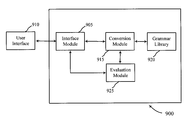
- the system includes an interface module 905 , that may provide an interface between a user interface 910 and one or more other modules.
- the interface module 905 may include one or more communications interfaces on a computer system, for example, that interact with one or more of a monitor, keyboard, and/or mouse of user interface 910 .
- a conversion module 915 is communicatively coupled to the interface module, and functions to convert received input into mathematical expressions and one or more ASTs.
- the conversion module 915 accesses a grammar library 920 , and evaluates received input relative to the grammar library to perform conversion functions.
- An evaluation module 925 evaluates the ASTs according to functions determined by the conversion module, and outputs results to the interface module 905 .
- the evaluation may be performed in intermediate steps, with the results of one or more intermediate steps output as well.
- various functions of the interface module 905 , conversion module 915 , grammar library 920 , and evaluation module 925 may be performed on a local system, or on a remote system connected to a local system through a network. Such a system 1000 is illustrated in FIG. 10 . In the embodiment of FIG.
- a user system 1010 is connected through a network 1015 to a central server computer system 1020 , that may perform some or all of the functions described above.
- the network 1015 may a local or wide area network, such as the Internet.
- the user system 1010 may include any of a number of user devices, such as a personal computer, tablet computer, handheld device, or other mobile device as are well known.
- FIGS. 11 and 12 illustrate screen shots of exemplary outputs that may be provided to a user of such systems.
- DSP digital signal processor
- ASIC application specific integrated circuit
- FPGA field programmable gate array
- a general-purpose processor may be a microprocessor, but in the alternative, the processor may be any conventional processor, controller, microcontroller, or state machine.
- a processor may also be implemented as a combination of computing devices, e.g., a combination of a DSP and a microprocessor, multiple microprocessors, one or more microprocessors in conjunction with a DSP core, or any other such configuration.
- the functions described herein may be implemented in hardware, software executed by a processor, firmware, or any combination thereof. If implemented in software executed by a processor, the functions may be stored on or transmitted over as one or more instructions or code on a computer-readable medium. Other examples and implementations are within the scope and spirit of the disclosure and appended claims. For example, due to the nature of software, functions described above can be implemented using software executed by a processor, hardware, firmware, hardwiring, or combinations of any of these. Features implementing functions may also be physically located at various positions, including being distributed such that portions of functions are implemented at different physical locations.
- Computer-readable media includes both computer storage media and communication media including any medium that facilitates transfer of a computer program from one place to another.
- a storage medium may be any available medium that can be accessed by a general purpose or special purpose computer.
- computer-readable media can comprise RAM, ROM, EEPROM, CD-ROM or other optical disk storage, magnetic disk storage or other magnetic storage devices, or any other medium that can be used to carry or store desired program code means in the form of instructions or data structures and that can be accessed by a general-purpose or special-purpose computer, or a general-purpose or special-purpose processor.
- any connection is properly termed a computer-readable medium.
- Disk and disc include compact disc (CD), laser disc, optical disc, digital versatile disc (DVD), floppy disk and blue-ray disc where disks usually reproduce data magnetically, while discs reproduce data optically with lasers. Combinations of the above are also included within the scope of computer-readable media.
Abstract
Description
-
- 1. Disconnection between computer languages employed by math software and the mathematical language; and
- 2. Inadequate communication between the software and student users.
The first factor is manifested by: A) Significant differences in syntax for symbolic expressions between the computer languages employed by math software and natural math notation; and B). Lack of systematic representation of the hybrid syntax in computer languages.
lim(f(x))@(x−>a^-)
Also note that in Table 1, f^(n)(x) means the nth-order derivative of f(x)w.r.t.x when n≧1; f^n(x) means the n-th power of f^(x) with f^−1(x) being reserved for the inverse of f, where f is a function.
| TABLE 1 |
| Summary of math notation and corresponding |
| one-dimensional expressions |
| Math notation | One-Dimensional Expression | Technique |
| α, β, γ, . . . | alpha, beta, gamma, . . . | Asciilization |
| ∫, ∂, ε, π, ∞, . . . | $, d, {, pi, inf, . . . | Asciilization |
|
|
lim(f(x) @(x − > a) | Leveling |
|
|
$f(x)dx @(a < x < b) $$f(x, y)dxdy@(a < x < b, g(x) < y < h(x)) | Leveling |
|
|
SUM(. . .) @(0 < i < m), PROD(. . .) @(0 < j < n) | Asciilization |
| ∇ f (x, y, z) | {grad|del|nabla}(f(x, y, z)) | Asciilization |
| ∇ × f (x, y, z) | {grad*|del*|nabla*}f(x, y, z)|curl(f(x, y, z)) | Asciilization |
| ∇ · f (x, y, z) | {grad.|del.|nabla.}f(x, y, z)|div(f(x, y, z)) | Asciilization |
| A × B | A * B | Asciilization |
| A · B | A · B | Adoption |
|
|
|
Leveling, unfolding |
|
|
|
Leveling, unfolding |
| <expr> = <expr> (1.1) | <expr> = <expr> (1.1) | Adoption |
|
|
d{circumflex over ( )}2f(x, y)/dxdy | Leveling |
|
|
(d/dx)(d/dy)f(x, y) | Operator transfor- mation |
| x′, y′, z′ | x′, y′, z′ | Adoption |
| f′ (x), f″ (x), f(n)(x) | f{circumflex over ( )}′(x), f{circumflex over ( )}″(x), f{circumflex over ( )}(n)(x) | Leveling |
| f′, f″ | f{circumflex over ( )}., f{circumflex over ( )}.. | Leveling |
| C*, a+, a− | C{circumflex over ( )}*(conjugate/adjoint op), a{circumflex over ( )}+, a{circumflex over ( )}− | Leveling |
| î, ĵ, {circumflex over (k)}, Â, | i{circumflex over ( )}{circumflex over ( )}, j{circumflex over ( )}{circumflex over ( )}, k{circumflex over ( )}{circumflex over ( )}(basic vecs), A{circumflex over ( )}{circumflex over ( )}(unit vec) | Leveling |
| !, |A|, ||A||, P(B|A) | !, |A|, ||A||, P(B|A) | Adoption |
| ai | a_i, a single symbol, or a[i] for 1D array | Leveling |
| aij | a[i][j], a is 2D array, matrix or tensor | |
where each pair of parenthesis is associated with one differentiation and thus the number of the pairs are the same as the order of derivatives. One embodiment simply applies the simple leveling technique to express the derivative as below
The syntax is a little difficult due to the distant pairing of parentheses, and another embodiment uses a variation of the above syntax:
In essence, the technique used above to level the derivative is operator-transformation. It is so-named because it changes the binary operator implied by the notation dg(x)/dx to a unary-prefix operator, where g(x) can be a function resulted from differentiation, namely, itself a derivative, as illustrated in
A→(V∪T)*
where * is the Kleen star operator, indicating zero or more of the elements belongs to the set it decorates. Then, the grammar is called a context-free grammar. Notice that there are no symbols around A, namely, the production rule for A that dictates how A is re-written, does not depend on its context, hence the name of context-free.
αAβ→αγβ
In the above rule, α,βε(V∪T)*, AεV, γε(V∪T)+, where + in the is the Kleen plus operator, indicating one or more of the elements belongs to the set it decorates. It seems that, from the above definitions, there is no direct link between whether the grammar is context-free and whether the interpretation can be context sensitive. As is well known, it is not desirable in a programming language to have ambiguities, i.e., multiple interpretations are possible from one statement or expression. As is also well known, ambiguities are not uncommon in natural languages such as Chinese and English. Ambiguities occur if multiple parse trees can be generated by a parser from a single sentence or statement using the chosen grammar. The assumption is that a parse tree of a statement/expression disassemblies the sentence into clearly defined structural units, from which a decisive interpretation can be obtained. It should be noted that context-dependency will not cause problem as long as the dependency can be resolved. This is indeed the case for embodiments herein. In one embodiment, the context-dependency is exclusively associated with operators. Namely, the interpretation of some of the operators depends on their context, i.e., their operands. Some concrete examples follow.
-
- <set>→{<set content>}
- <relation>→<expression><relation op><expression>
- <relation op>→{|>| . . .
The abstract-syntax-tree representing statement in natural math notation A={x|xε, x2>9} is displayed in
FIG. 5 . The hybrid statement for this notation would be “A={x|x{Real, x^2>9}”. The set qualifying sign | is necessary to differentiate the set-builder notation from the list notation used for defining sets.
| TABLE 2 |
| Summary of hybrid syntactic structures in natural language and |
| symbolic expressions |
| Syntactic Structures | Example |
| Assertion | a-statement | A is a 4 * 4 upper-triangular matrix; |
| the-statement | P is the tangent plane of S at x = a, y = b; | |
| descriptive- | f(x) is differentiable at x = 0; | |
| statement | ||
| Command | Calculate the distance between B and P; | |
| Solve x, y from (1.1), (1.2); | ||
| Query | Is f(x) continuous over 0 < x <= 1? | |
| Deduction | Given|Assuming <Assertions>, show|prove | |
| <Assertion>; | ||
| f(x,y) = ln(x−a)*sin(2*pi*y); | //definition | ||
| Is f(x,y) continuous at x = a, 0<= y < pi? | //query | ||
| Is f(x,y) periodic? | //query | ||
| A = (x_0, y_0, z_0); | //assignment | ||
| S = {(x,y,z)|z=x{circumflex over ( )}2+y{circumflex over ( )}2}; | //assignment | ||
| P is the tangent plane of S at x = 0, y = h; | //assertion | ||
| calculate the distance between P and A; | //command | ||
-
- begin
3x−4y+2z=0.3; (1.1)
13x+2y−34z=1.5; (1.2)
−5x−12y+0.1z=10.9; (1.3) - Solve x,y,z from (1.1)-(1.3);
- end#
The one-dimensional statements, and the command statement, are processed and, in this example, an interpreted input is displayed that may be used to verify the input was interpreted correctly.
- begin
3x−4y+2z=0.3 (1.1)
(13x+2y)−34z=1.5 (1.2)
−5x−12y+0.1z=10.9 (1.3)
As mentioned above, in some embodiments intermediate steps may be calculated and displayed to a user. In this example, a series of intermediate results are displayed to a user as follows.
Intermediate Steps:
To solve the linear system, we use the Gauss-Jordon elimination method. Let's first write the above set of linear equations in the following matrix form:
The Gauss-Jordon method applies a series of elementary row operations to both the coefficient matrix (A) and the column matrix on the right-hand-side (b) simultaneously until A becomes identity matrix (I). Then, the un-known column matrix is the same as b.
There are two types of elementary row operations involved here. One is row swapping represented by ri
Listed below are the sequence of the elementary row operations performed. Notice that the current pivot element is highlighted using boldface font for clarity.
Dividing each row of the coefficient matrix A and the column matrix b by the diagonal element aii, the system becomes:
As can be seen, now the coefficient matrix A is an identity matrix and we have:
The “Intermediate Steps” of this embodiment are created by a “solution composer.” Providing such a display of partial results may provide pedagogical value to student, and other users. In some embodiments, a user may not desire to view this sometimes lengthy and/or verbose section of output, and the display of such intermediate results can be turned off by the user. It worthwhile to point out that the whole linear system instead of the augmented matrix is displayed in the step-by-step illustration of the solving process with the hope that doing so would be more intuitive for student users, for example, to understand the operations involved. While row swapping is important for many practical applications, it could be a distraction to users, and may be turned off in various embodiments.
-
- <pre-formulae narrative><formula list><post-formulae narratives>
The <pre-formulae narrative> normally contains descriptions about procedures and assumptions leading to the formulae—mathematical/quantitative statements about name entities appeared in the text; and <post-formulae narrative> provides explanations about the symbols representing the name entities and further elaborations about the equations. This structure is used in the construction of “Intermediate Steps” in this example.
- <pre-formulae narrative><formula list><post-formulae narratives>
x^2−exp(x)=sin(x)+0.3; (1.1)
x 2 −e x=sin(x)+0.3 (1.1)
x=−0.5703899316
x 2 −e x=sin(x)+0.3
numerically with the Newton-Raphson method. First, let's transform the equation into a standardized form:
ƒ(x)=(x 2 −e x)−(sin(x)+0.3)=0
ƒ(x)=ƒ(x k)+ƒ′(x k)(x−x k), k≧0
where ƒ′(xk) is the derivative of ƒ with respect to x evaluated at x=xk
| k | xk | f(xk) | (df/dx)x=x k | |xk − xk−1| |
| 0 | 1.00000000 | −2.85975281 | −1.25858413 | N.A. |
| 1 | −1.27219837 | 1.99402363 | −3.11879216 | 2.2722e+000 |
| 2 | −0.63284071 | 0.16084411 | −2.60311309 | 6.3936e−001 |
| 3 | −0.57105158 | 0.00168592 | −2.54836726 | 6.1789e−002 |
| 4 | −0.57039001 | 0.00000020 | −2.54777539 | 6.6157e−004 |
| 5 | −0.57038993 | 0.00000000 | −2.54777532 | 7.6841e−008 |
ƒ(x)=∫x 3(1−x 2)dx
p(x)=ƒx cos(x 2)dx
q(x)=∫ sin3(x)cos2(x)dx
-
- §Notice the integrand of integral ∫x3(1−x2)dx contains product that can be further expanded, so let's try expanding the integrand and then integrating term-by-term:
x 3(1−x 2)=x 3 −x 5
- §Notice the integrand of integral ∫x3(1−x2)dx contains product that can be further expanded, so let's try expanding the integrand and then integrating term-by-term:
∫(x 3 −x 5)dx=∫x 3 dx−∫x 5 dx
-
- §Applying the additive rule of integration, we have
∫κe −βx dx=κ∫e −βx dx
u=−βx
and
Therefore
contains pattern √{square root over (a2−x2)}.
x=a sin(φ), −π/2≦φ≦+π/2
√{square root over (a 2 −x 2)}=|a| cos(φ)
and
back to the above result gives
-
- §To evaluate indefinite integral ∫x cos(x2)dx, let's try substitution
u=x2
- §To evaluate indefinite integral ∫x cos(x2)dx, let's try substitution
and
-
- §Notice that the integrand of integral ƒ sin (x)3 cos (x)2dx contains pattern sin(x)m. Applying trigonometric identity
sin(x)2=1−cos(x)2
to the integrand gives:
- §Notice that the integrand of integral ƒ sin (x)3 cos (x)2dx contains pattern sin(x)m. Applying trigonometric identity
u=cos(x)
and
∫(u 2 −u 4)du=∫u 2 du−∫u 4 du
A=aî+bĵ+c{circumflex over (k)}
r=xîyĵ+z{circumflex over (k)}
T s =A·B×r
C=(αî+βĵ)×Â
D=∇X B
E=|B|∇·B
A=aî+bĵ+c{circumflex over (k)}
r=xî+yĵ+z{circumflex over (k)}
where Ax, Ay, Az are the components of the vector, and |A| is the length of the vector:
|A|=√{square root over (a 2 +b 2)}+c 2
thus
-
- (0 c h^2)
- (x y z);
-
- (0, 1, 0)
- (0, 0, 1);
B=|A T −κI|
B=(a−κ)((c−κ)(z−κ)−yh 2)+x(2h 2−(c−κ)ψ
| T = |
| k | x; | | sigma | ||
| 1 | 0.00 | 3.391130 | 0.169556 | ||
| 2 | 0.20 | 3.485675 | 0.174284 | ||
| 3 | 0.40 | 4.224254 | 0.211213 | ||
| 4 | 0.60 | 4.307524 | 0.215376 | ||
| 5 | 0.80 | 4.261938 | 0.213097 | ||
| 6 | 1.00 | 4.588840 | 0.229442 | ||
| 7 | 1.20 | 4.849868 | 0.242493 | ||
| 8 | 1.40 | 4.868594 | 0.243430 | ||
| 9 | 1.60 | 4.768181 | 0.238409 | ||
| 10 | 1.80 | 4.803114 | 0.240156 | ||
| 11 | 2.00 | 4.931015 | 0.246551 | ||
| 12 | 2.20 | 4.810400 | 0.240520 | ||
| 13 | 2.40 | 5.082588 | 0.254129 | ||
| 14 | 2.60 | 5.037386 | 0.251869 | ||
| 15 | 2.80 | 4.476670 | 0.223833 | ||
| 16 | 3.00 | 4.379418 | 0.218971 | ||
| 17 | 3.20 | 4.665796 | 0.233290 | ||
| 18 | 3.4 | 4.201536 | 0.210077 | ||
| 19 | 3.60 | 3.705798 | 0.185290 | ||
| 20 | 3.80 | 3.238404 | 0.161920; | ||
| TABLE 1 |
| Input tabular data. |
| k | | y | σ | ||
| 1 | 0.0 | 3.39113 | 0.169556 | ||
| 2 | 0.2 | 3.485675 | 0.174284 | ||
| 3 | 0.4 | 4.224254 | 0.211213 | ||
| 4 | 0.6 | 4.307524 | 0.215376 | ||
| 5 | 0.8 | 4.261938 | 0.213097 | ||
| 6 | 1.0 | 4.58884 | 0.229442 | ||
| 7 | 1.2 | 4.849868 | 0.242493 | ||
| 8 | 1.4 | 4.868594 | 0.24343 | ||
| 9 | 1.6 | 4.768181 | 0.238409 | ||
| 10 | 1.8 | 4.803114 | 0.240156 | ||
| 11 | 2.0 | 4.931015 | 0.246551 | ||
| 12 | 2.2 | 4.8104 | 0.24052 | ||
| 13 | 2.4 | 5.082588 | 0.254129 | ||
| 14 | 2.6 | 5.037386 | 0.251869 | ||
| 15 | 2.8 | 4.47667 | 0.223833 | ||
| 16 | 3.0 | 4.379418 | 0.218971 | ||
| 17 | 3.2 | 4.665796 | 0.23329 | ||
| 18 | 3.4 | 4.201536 | 0.210077 | ||
| 19 | 3.6 | 3.705798 | 0.18529 | ||
| 20 | 3.8 | 3.238404 | 0.16192 | ||
κ=√{square root over (<y 2 >−<y>2)}
κ=0.5448777363
the model parameters are estimated to be:
and
χ2=14.594367981
| TABLE 2 |
| Comparsion of input data and fit. |
| k | x | y | σ | f(x) |
| 1.000000 | 0.000000 | 3.391130 | 0.169556 | 3.383717 |
| 2.000000 | 0.200000 | 3.485675 | 0.174284 | 3.656025 |
| 3.000000 | 0.400000 | 4.224254 | 0.211213 | 3.916922 |
| 4.000000 | 0.600000 | 4.307524 | 0.215376 | 4.161035 |
| 5.000000 | 0.800000 | 4.261938 | 0.213097 | 4.383070 |
| 6.000000 | 1.000000 | 4.588840 | 0.229442 | 4.578002 |
| 7.000000 | 1.200000 | 4.849868 | 0.242493 | 4.741266 |
| 8.000000 | 1.400000 | 4.868594 | 0.243430 | 4.868927 |
| 9.000000 | 1.600000 | 4.768181 | 0.238409 | 4.957845 |
| 10.000000 | 1.800000 | 4.803114 | 0.240156 | 5.005796 |
| 11.000000 | 2.000000 | 4.931015 | 0.246551 | 5.011573 |
| 12.000000 | 2.200000 | 4.810400 | 0.240520 | 4.975029 |
| 13.000000 | 2.400000 | 5.082588 | 0.254129 | 4.897086 |
| 14.000000 | 2.600000 | 5.037386 | 0.251869 | 4.779699 |
| 15.000000 | 2.800000 | 4.476670 | 0.223833 | 4.625770 |
| 16.000000 | 3.000000 | 4.379418 | 0.218971 | 4.439030 |
| 17.000000 | 3.200000 | 4.665796 | 0.233290 | 4.223892 |
| 18.000000 | 3.400000 | 4.201536 | 0.210077 | 3.985274 |
| 19.000000 | 3.600000 | 3.705798 | 0.185290 | 3.728415 |
| 20.000000 | 3.800000 | 3.238404 | 0.161920 | 3.458684 |
where
| TABLE 3 |
| Iteration results. |
| step | a | μ | b | χ2(a, μ, b) |
| 0 | 0.500000 | 0.500000 | 0.500000 | 7601.939941 |
| 1 | 3.382416 | 1.533874 | 4.992346 | 611.439758 |
| 2 | 4.937086 | 2.878956 | −0.464357 | 5814.545898 |
| 3 | 4.932500 | 2.872879 | −0.422426 | 6020.951660 |
| 4 | 4.888673 | 2.815298 | −0.024240 | 7628.460938 |
| 5 | 4.585768 | 2.447740 | 2.565272 | 406.553802 |
| 6 | 4.838821 | 2.026784 | 3.151937 | 25.881390 |
| 7 | 5.010530 | 1.919288 | 3.067020 | 14.638807 |
| 8 | 5.014384 | 1.927227 | 3.072919 | 14.594368 |
| 9 | 5.014555 | 1.927224 | 3.072608 | 14.594371 |
A=∫ 0 1∫0 2∫0 x(x+y+1)dydzdx
A=2
∫x=0 1∫z=0 2∫y=0 x(x+y+1)dydzdx=∫ x=0 1(∫z=0 2∫y=0 x(x+y+1)dydz)dx
∫z=0 2∫y=0 x(x+y+1)dydz=∫ z=0 2(∫y=0 x(x+y+1)dy)dz
-
- §To evaulate the definite integral ∫0 x(x+y+1)dy, let's first work out the indefinite integral ∫(x+y+1)dy. Applying the additive rule of integration, we have
∫x=0 1(x+y+1)dy=∫xdy+∫ydy+∫1dy
∫xdy=yx
- §To evaulate the definite integral ∫0 x(x+y+1)dy, let's first work out the indefinite integral ∫(x+y+1)dy. Applying the additive rule of integration, we have
∫1dy=y
-
- §To evaluate the definite integral
let's first work out the indefinite integral
-
- §To evaluate the definite integral
let's first work out the indefinite integral
Factoring out x-independent factor
∫0 1∫0 2∫0 x(x+y+1)dydzdx=2
ρ(x,y)=x+y 2
C={(x,y)|x=t, y=t, 0<t<1}
ds=√{square root over ((dx)2+(dy)2)}{square root over ((dx)2+(dy)2)}
m=∫ Cρ(x,y)ds
ρ(x,y)=x+y 2
C={(x,y)|x=t, y=t, 0<t<1}
ds=√{square root over (dx 2+dy 2)}
x=t
y=t
from the curve definition into ρ(x,y), we obtain
ρ(x,y)=t+t 2
-
- §To evaluate the definite integral ∫0 1(t+t2)√{square root over (2)}dt, let's first work out the indefinite integral ∫(t+t2)√{square root over (2 )}dt. Factoring out t-independent factor
∫(t+t 2)√{square root over (2)}dt=√{square root over (2)}∫((t+t 2))dt
- §To evaluate the definite integral ∫0 1(t+t2)√{square root over (2)}dt, let's first work out the indefinite integral ∫(t+t2)√{square root over (2 )}dt. Factoring out t-independent factor
∫((t+t 2))dt=∫tdt+∫t 2 dt
C={(x,y,z)|x=cos(t), y=sin(t), z=t, 0<t<π}
F=yî+xĵ
r=xî+yĵ+z{circumflex over (k)}
N=∫ cF×dr
C={(x,y,z)|x=cos(t), y=sin(t), z=t, 0<t<π}
F=yî+xĵ
r=xî+yĵ+z{circumflex over (k)}
N=(−2)ĵ
-
- ∫CF×dr is a line integral along curve C. To compute it, we need to first work out F and differential dr along the curve in terms of parameter t. Plugging
x=cos(t)
y=sin(t)
z=t
From the curve definition into (yî+xĵ), we obtain
- ∫CF×dr is a line integral along curve C. To compute it, we need to first work out F and differential dr along the curve in terms of parameter t. Plugging
and
-
- §To evaluate the definite integral ∫0 π cos(t) dt, let's first work out the indefinite integral ∫ cos(t)dt.
∫cos(t)dt=sin(t)
- §To evaluate the definite integral ∫0 π cos(t) dt, let's first work out the indefinite integral ∫ cos(t)dt.
-
- §To evaluate the definite integral ∫0 π sin(t)dt, let's first work out the indefinite integral ∫−sin(t)dt.
∫ sin(t)dt=−cos(t)
- §To evaluate the definite integral ∫0 π sin(t)dt, let's first work out the indefinite integral ∫−sin(t)dt.
-
- §To evaluate the definite integral ∫0 π2 sin(t)cos(t) dt, let's first work out the indefinite integral ∫2 sin(t)cos(t)dt. Factoring out t-independent factor
∫2 sin(t)cos(t)dt=2∫ sin(t)cos(t)dt
- §To evaluate the definite integral ∫0 π2 sin(t)cos(t) dt, let's first work out the indefinite integral ∫2 sin(t)cos(t)dt. Factoring out t-independent factor
u=sin(t)
and
y^2−4*y=x^2*(x^2−4); (1.1)
y 2−4y=x 2(x 2−4) (1.1)
calculate
from 1.1.
y 2−4y=x 2(x 2−4)
let's take derivatives with respect to x for both sides of the above equation. Applying additive rule
-
- (−sin(phi)cos(phi));
-
- For i=1, j=2:
-
- Therefore the matrix is not; orthogonal.
S={(x,y,z)|z=x, 0<x<R, 0<y<x}
u=u0z{circumflex over (k)}
n=((d/dx)z,(d/dy)z,(−1))
Q=∫ S u·{circumflex over (n)}dS
S={(x,y,z)|0<x<R, 0<y<x, z=x}
u=u0z{circumflex over (k)}
n=(d/dx)zî+(d/dy)zĵ+{circumflex over (k)}
z=x
from the surface definition into (u0z{circumflex over (k)})·{circumflex over (n)}, we have
(u 0 z{circumflex over (k)})=u 0 x{circumflex over (k)}
((d/dx)zî+(d/dy)zĵ−{circumflex over (k)})=î−{circumflex over (k)}
and
thus,
dS=√{square root over ((∂z/∂x)2+(∂z/∂y)2+1)}{square root over ((∂z/∂x)2+(∂z/∂y)2+1)}dxdy
z=x
into the above equation, we obtain
dS=√{square root over (2)}dxdy.
D={(x,y)|0<x<R, 0<y<x},
we can express the surface integral as a double integral defined in region D as below:
∫x=0 R∫y=0 x −u 0 xdydx=∫ x=0 R(∫y=0 x −u 0 xdy)dx
-
- ÅTo evaluate the definite integral ∫0 x−u0xdy, let's first work out the indefinite integral ∫−u0xdy.
∫−u 0 xdy=−yu 0 x
- ÅTo evaluate the definite integral ∫0 x−u0xdy, let's first work out the indefinite integral ∫−u0xdy.
-
- ÅTo evaluate the definite integral ∫0 R−x2u0dx, let's first work out the indefinite integral ∫−x2u0dx. Factoring out x-independent factor
A=(x 0 ,y 0 ,z 0)
S={(x,y,z)|z=x 2 +y 2, 0<x<∞, 0<y<x}
A=x 0 î+y 0 ĵ+z 0 {circumflex over (k)}
S={(x,y,z)|0<x<∞, 0<y<x, z=(x 2 +y 2)}
P={(x,y,z)|Ax+By+Cz+D=0,xε
where
{circumflex over (n)}·((x−x′){circumflex over (i)}+(y−y′){circumflex over (j)}+(z−z′)=0
z=x 2 +y 2
we have:
and
or equivalently,
Ax+By+Cz+D=0
A=0
where A, B, C, D are the coefficients defining the plane. Plugging the coefficients defining the plane and the coordinates of the point (x0, y0, z0) into the formula, we obtain:
Claims (35)
Priority Applications (2)
| Application Number | Priority Date | Filing Date | Title |
|---|---|---|---|
| US13/188,090 US8943113B2 (en) | 2011-07-21 | 2011-07-21 | Methods and systems for parsing and interpretation of mathematical statements |
| PCT/US2012/047650 WO2013013173A2 (en) | 2011-07-21 | 2012-07-20 | Methods and systems for parsing and interpretation of mathematical statements |
Applications Claiming Priority (1)
| Application Number | Priority Date | Filing Date | Title |
|---|---|---|---|
| US13/188,090 US8943113B2 (en) | 2011-07-21 | 2011-07-21 | Methods and systems for parsing and interpretation of mathematical statements |
Publications (2)
| Publication Number | Publication Date |
|---|---|
| US20130024487A1 US20130024487A1 (en) | 2013-01-24 |
| US8943113B2 true US8943113B2 (en) | 2015-01-27 |
Family
ID=47556556
Family Applications (1)
| Application Number | Title | Priority Date | Filing Date |
|---|---|---|---|
| US13/188,090 Expired - Fee Related US8943113B2 (en) | 2011-07-21 | 2011-07-21 | Methods and systems for parsing and interpretation of mathematical statements |
Country Status (2)
| Country | Link |
|---|---|
| US (1) | US8943113B2 (en) |
| WO (1) | WO2013013173A2 (en) |
Cited By (4)
| Publication number | Priority date | Publication date | Assignee | Title |
|---|---|---|---|---|
| US20180357207A1 (en) * | 2017-06-13 | 2018-12-13 | Microsoft Technology Licensing, Llc | Evaluating documents with embedded mathematical expressions |
| US11080359B2 (en) | 2017-12-21 | 2021-08-03 | International Business Machines Corporation | Stable data-driven discovery of a symbolic expression |
| US11379553B2 (en) | 2018-01-10 | 2022-07-05 | International Business Machines Corporation | Interpretable symbolic decomposition of numerical coefficients |
| US11599829B2 (en) | 2020-04-29 | 2023-03-07 | International Business Machines Corporation | Free-form integration of machine learning model primitives |
Families Citing this family (17)
| Publication number | Priority date | Publication date | Assignee | Title |
|---|---|---|---|---|
| US8777731B2 (en) * | 2012-02-08 | 2014-07-15 | Wms Gaming, Inc. | Dynamic configuration of wagering games |
| US9460075B2 (en) | 2014-06-17 | 2016-10-04 | International Business Machines Corporation | Solving and answering arithmetic and algebraic problems using natural language processing |
| US9514185B2 (en) * | 2014-08-07 | 2016-12-06 | International Business Machines Corporation | Answering time-sensitive questions |
| US9430557B2 (en) | 2014-09-17 | 2016-08-30 | International Business Machines Corporation | Automatic data interpretation and answering analytical questions with tables and charts |
| US10102276B2 (en) | 2015-12-07 | 2018-10-16 | International Business Machines Corporation | Resolving textual numerical queries using natural language processing techniques |
| KR101842873B1 (en) * | 2016-09-29 | 2018-03-28 | 조봉한 | A mathematical translator, mathematical translation device and its platform |
| US10592213B2 (en) * | 2016-10-19 | 2020-03-17 | Intel Corporation | Preprocessing tensor operations for optimal compilation |
| US10706215B2 (en) * | 2017-04-05 | 2020-07-07 | Parsegon | Producing formula representations of mathematical text |
| US11010401B2 (en) * | 2017-04-25 | 2021-05-18 | Microsoft Technology Licensing, Llc | Efficient snapshot generation of data tables |
| US10162613B1 (en) * | 2017-07-18 | 2018-12-25 | Sap Portals Israel Ltd. | Re-usable rule parser for different runtime engines |
| CN110069743B (en) * | 2019-04-29 | 2023-02-24 | 武汉轻工大学 | Multi-mode calculus calculation method, device, equipment and storage medium |
| US11243948B2 (en) | 2019-08-08 | 2022-02-08 | Salesforce.Com, Inc. | System and method for generating answers to natural language questions based on document tables |
| US11347733B2 (en) | 2019-08-08 | 2022-05-31 | Salesforce.Com, Inc. | System and method for transforming unstructured numerical information into a structured format |
| US11106668B2 (en) | 2019-08-08 | 2021-08-31 | Salesforce.Com, Inc. | System and method for transformation of unstructured document tables into structured relational data tables |
| US11861308B2 (en) | 2020-04-15 | 2024-01-02 | Intuit Inc. | Mapping natural language utterances to operations over a knowledge graph |
| US20220207238A1 (en) * | 2020-12-30 | 2022-06-30 | International Business Machines Corporation | Methods and system for the extraction of properties of variables using automatically detected variable semantics and other resources |
| US20240104292A1 (en) * | 2022-09-23 | 2024-03-28 | Texas Instruments Incorporated | Mathematical calculations with numerical indicators |
Citations (17)
| Publication number | Priority date | Publication date | Assignee | Title |
|---|---|---|---|---|
| US4736320A (en) | 1985-10-08 | 1988-04-05 | Foxboro Company | Computer language structure for process control applications, and translator therefor |
| US5247693A (en) | 1985-10-08 | 1993-09-21 | The Foxboro Company | Computer language structure for process control applications and method of translating same into program code to operate the computer |
| US5355496A (en) | 1992-02-14 | 1994-10-11 | Theseus Research, Inc. | Method and system for process expression and resolution including a generally and inherently concurrent computer language |
| US5878386A (en) | 1996-06-28 | 1999-03-02 | Microsoft Corporation | Natural language parser with dictionary-based part-of-speech probabilities |
| US6058385A (en) | 1988-05-20 | 2000-05-02 | Koza; John R. | Simultaneous evolution of the architecture of a multi-part program while solving a problem using architecture altering operations |
| US6101556A (en) | 1997-01-07 | 2000-08-08 | New Era Of Networks, Inc. | Method for content-based dynamic formatting for interoperation of computing and EDI systems |
| US20020126905A1 (en) * | 2001-03-07 | 2002-09-12 | Kabushiki Kaisha Toshiba | Mathematical expression recognizing device, mathematical expression recognizing method, character recognizing device and character recognizing method |
| US20040015342A1 (en) | 2002-02-15 | 2004-01-22 | Garst Peter F. | Linguistic support for a recognizer of mathematical expressions |
| US20060005115A1 (en) | 2004-06-30 | 2006-01-05 | Steven Ritter | Method for facilitating the entry of mathematical expressions |
| US20060085781A1 (en) * | 2004-10-01 | 2006-04-20 | Lockheed Martin Corporation | Library for computer-based tool and related system and method |
| US7165113B2 (en) | 2000-11-28 | 2007-01-16 | Hewlett-Packard Development Company, L.P. | Computer language for defining business conversations |
| US7272543B2 (en) | 2001-10-18 | 2007-09-18 | Infineon Technologies Ag | Method and computer system for structural analysis and correction of a system of differential equations described by a computer language |
| US20080091409A1 (en) | 2006-10-16 | 2008-04-17 | Microsoft Corporation | Customizable mathematic expression parser and evaluator |
| US20080263403A1 (en) | 2004-09-18 | 2008-10-23 | Andrei Nikolaevich Soklakov | Conversion of Mathematical Statements |
| US7636697B1 (en) * | 2007-01-29 | 2009-12-22 | Ailive Inc. | Method and system for rapid evaluation of logical expressions |
| US20100281350A1 (en) | 2009-04-29 | 2010-11-04 | Nokia Corporation | Method, Apparatus, and Computer Program Product for Written Mathematical Expression Analysis |
| WO2011038445A1 (en) | 2009-09-29 | 2011-04-07 | Zap Holdings Ldt | A content based approach to extending the form and function of a business intelligence system |
-
2011
- 2011-07-21 US US13/188,090 patent/US8943113B2/en not_active Expired - Fee Related
-
2012
- 2012-07-20 WO PCT/US2012/047650 patent/WO2013013173A2/en active Application Filing
Patent Citations (18)
| Publication number | Priority date | Publication date | Assignee | Title |
|---|---|---|---|---|
| US5247693A (en) | 1985-10-08 | 1993-09-21 | The Foxboro Company | Computer language structure for process control applications and method of translating same into program code to operate the computer |
| US4736320A (en) | 1985-10-08 | 1988-04-05 | Foxboro Company | Computer language structure for process control applications, and translator therefor |
| US6058385A (en) | 1988-05-20 | 2000-05-02 | Koza; John R. | Simultaneous evolution of the architecture of a multi-part program while solving a problem using architecture altering operations |
| US5355496A (en) | 1992-02-14 | 1994-10-11 | Theseus Research, Inc. | Method and system for process expression and resolution including a generally and inherently concurrent computer language |
| US5878386A (en) | 1996-06-28 | 1999-03-02 | Microsoft Corporation | Natural language parser with dictionary-based part-of-speech probabilities |
| US6101556A (en) | 1997-01-07 | 2000-08-08 | New Era Of Networks, Inc. | Method for content-based dynamic formatting for interoperation of computing and EDI systems |
| US7165113B2 (en) | 2000-11-28 | 2007-01-16 | Hewlett-Packard Development Company, L.P. | Computer language for defining business conversations |
| US20020126905A1 (en) * | 2001-03-07 | 2002-09-12 | Kabushiki Kaisha Toshiba | Mathematical expression recognizing device, mathematical expression recognizing method, character recognizing device and character recognizing method |
| US7272543B2 (en) | 2001-10-18 | 2007-09-18 | Infineon Technologies Ag | Method and computer system for structural analysis and correction of a system of differential equations described by a computer language |
| US20040015342A1 (en) | 2002-02-15 | 2004-01-22 | Garst Peter F. | Linguistic support for a recognizer of mathematical expressions |
| US7373291B2 (en) | 2002-02-15 | 2008-05-13 | Mathsoft Engineering & Education, Inc. | Linguistic support for a recognizer of mathematical expressions |
| US20060005115A1 (en) | 2004-06-30 | 2006-01-05 | Steven Ritter | Method for facilitating the entry of mathematical expressions |
| US20080263403A1 (en) | 2004-09-18 | 2008-10-23 | Andrei Nikolaevich Soklakov | Conversion of Mathematical Statements |
| US20060085781A1 (en) * | 2004-10-01 | 2006-04-20 | Lockheed Martin Corporation | Library for computer-based tool and related system and method |
| US20080091409A1 (en) | 2006-10-16 | 2008-04-17 | Microsoft Corporation | Customizable mathematic expression parser and evaluator |
| US7636697B1 (en) * | 2007-01-29 | 2009-12-22 | Ailive Inc. | Method and system for rapid evaluation of logical expressions |
| US20100281350A1 (en) | 2009-04-29 | 2010-11-04 | Nokia Corporation | Method, Apparatus, and Computer Program Product for Written Mathematical Expression Analysis |
| WO2011038445A1 (en) | 2009-09-29 | 2011-04-07 | Zap Holdings Ldt | A content based approach to extending the form and function of a business intelligence system |
Non-Patent Citations (1)
| Title |
|---|
| International Search Report, PCT/US2012/047650 dated Jul. 30, 2013. |
Cited By (5)
| Publication number | Priority date | Publication date | Assignee | Title |
|---|---|---|---|---|
| US20180357207A1 (en) * | 2017-06-13 | 2018-12-13 | Microsoft Technology Licensing, Llc | Evaluating documents with embedded mathematical expressions |
| US10540424B2 (en) * | 2017-06-13 | 2020-01-21 | Microsoft Technology Licensing, Llc | Evaluating documents with embedded mathematical expressions |
| US11080359B2 (en) | 2017-12-21 | 2021-08-03 | International Business Machines Corporation | Stable data-driven discovery of a symbolic expression |
| US11379553B2 (en) | 2018-01-10 | 2022-07-05 | International Business Machines Corporation | Interpretable symbolic decomposition of numerical coefficients |
| US11599829B2 (en) | 2020-04-29 | 2023-03-07 | International Business Machines Corporation | Free-form integration of machine learning model primitives |
Also Published As
| Publication number | Publication date |
|---|---|
| WO2013013173A3 (en) | 2013-10-31 |
| WO2013013173A2 (en) | 2013-01-24 |
| US20130024487A1 (en) | 2013-01-24 |
Similar Documents
| Publication | Publication Date | Title |
|---|---|---|
| US8943113B2 (en) | Methods and systems for parsing and interpretation of mathematical statements | |
| Oh | Symplectic topology and Floer homology | |
| Marin et al. | Bayesian essentials with R | |
| Hjorth-Jensen | Computational physics | |
| Nyamoradi et al. | On boundary value problems for impulsive fractional differential equations | |
| Meduna | Elements of compiler design | |
| Ye et al. | Visually dynamic presentation of proofs in plane geometry: Part 1. Basic features and the manual input method | |
| Cramer et al. | Parsing and disambiguation of symbolic mathematics in the Naproche system | |
| Kaisare | Computational techniques for process simulation and analysis using Matlab® | |
| Anastassiou et al. | Numerical analysis using sage | |
| Marché | Verification of the functional behavior of a floating-point program: an industrial case study | |
| Kang et al. | Analyticalink: An interactive learning environment for math word problem solving | |
| Bientinesi et al. | Deriving dense linear algebra libraries | |
| Asakura et al. | Miogatto: A math identifier-oriented grounding annotation tool | |
| Heys | Chemical and biomedical engineering calculations using Python | |
| Biletch et al. | An Analysis of Mathematical Notations: For Better or For Worse | |
| Senese | Symbolic Mathematics for Chemists: A Guide for Maxima Users | |
| Üçoluk et al. | Introduction to programming concepts with case studies in Python | |
| Oh | Symplectic Topology and Floer Homology: Volume 2, Floer Homology and its Applications | |
| Lapets | User-friendly Support for Common Concepts in a Lightweight Verifier | |
| Li et al. | H❤️ rtDown: Document Processor for Executable Linear Algebra Papers | |
| Nederhof et al. | A customized grammar workbench | |
| Omar | Reasonably programmable syntax | |
| Huet et al. | Sanskrit linguistics web services | |
| Lambers et al. | Explorations in numerical analysis: Python edition |
Legal Events
| Date | Code | Title | Description |
|---|---|---|---|
| STCF | Information on status: patent grant |
Free format text: PATENTED CASE |
|
| MAFP | Maintenance fee payment |
Free format text: PAYMENT OF MAINTENANCE FEE, 4TH YR, SMALL ENTITY (ORIGINAL EVENT CODE: M2551) Year of fee payment: 4 |
|
| FEPP | Fee payment procedure |
Free format text: MAINTENANCE FEE REMINDER MAILED (ORIGINAL EVENT CODE: REM.); ENTITY STATUS OF PATENT OWNER: SMALL ENTITY |
|
| LAPS | Lapse for failure to pay maintenance fees |
Free format text: PATENT EXPIRED FOR FAILURE TO PAY MAINTENANCE FEES (ORIGINAL EVENT CODE: EXP.); ENTITY STATUS OF PATENT OWNER: SMALL ENTITY |
|
| STCH | Information on status: patent discontinuation |
Free format text: PATENT EXPIRED DUE TO NONPAYMENT OF MAINTENANCE FEES UNDER 37 CFR 1.362 |
|
| FP | Lapsed due to failure to pay maintenance fee |
Effective date: 20230127 |